The Problem of Visualizing Data in High Dimensions

Visualizing data in spaces with more than three dimensions is a challenging task, particularly in the context of many-objective optimization. The goal of such visualizations may vary depending on the context:

• In some cases, the aim is to display the distribution of the dataset in the input space;
• In others, it is useful to visualize the Efficient Set (or Pareto front) in the output space.

There are also specific techniques designed to visualize input-output relationships, both in single-objective and multi-objective scenarios. Below, we discuss several of these methods, each with its own strengths and limitations.

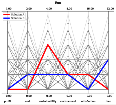
Parallel Coordinates

Parallel Coordinates is a widely-used and intuitive method for visualizing high-dimensional data. Each objective is represented as a vertical axis, and all axes are aligned side by side. A solution is visualized as a line that connects its values across the different axes.

This method is particularly helpful for observing dominance relationships: if one line is consistently lower (in a minimization problem) than another and does not intersect it, it dominates the other. If two lines intersect, the corresponding solutions are non-dominated

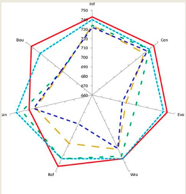
The Radar Chart (or spider plot) is a visual variation of parallel coordinates. Here, each objective corresponds to a radial axis emanating from the center of a regular polygon. A solution is represented as a polygonal shape connecting the values on these axes.

In minimization problems, a solution that is more “internal” is generally better. If two solutions intersect, it indicates they are non-dominated.

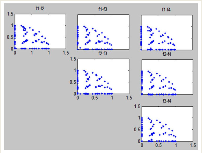
The Scatterplot Matrix (or SPLOM) shows all pairwise combinations of objectives using standard 2D scatterplots. It is useful for detecting correlations between objectives, but it does not scale well with a high number of dimensions.

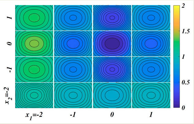
The Tile Plot resembles a scatterplot but uses contour plots or color gradients to represent density or other characteristics of the data. It provides insight into global structures or data distribution patterns.

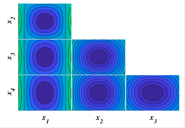
The Nested Axes Plot is particularly effective when visualizing 4D or 5D data, especially if some variables are discrete. Discrete variables (e.g., ( x_1 ), ( x_2 )) are used to define a grid layout, while continuous variables are plotted within each grid cell. This method allows analysts to explore dependencies and trends in moderately high-dimensional spaces.

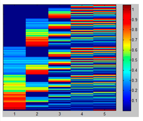
A Heatmap represents objective values through color intensity. Each row corresponds to a solution, and each column to an objective. While similar in spirit to parallel coordinates, it encodes the information differently.

Heatmaps are:

• Easy to construct;
• Scalable with respect to the number of objectives;
• Useful to highlight correlations or clusters.

However, they do not scale well with a large number of solutions, and cannot preserve the shape of the Pareto front.

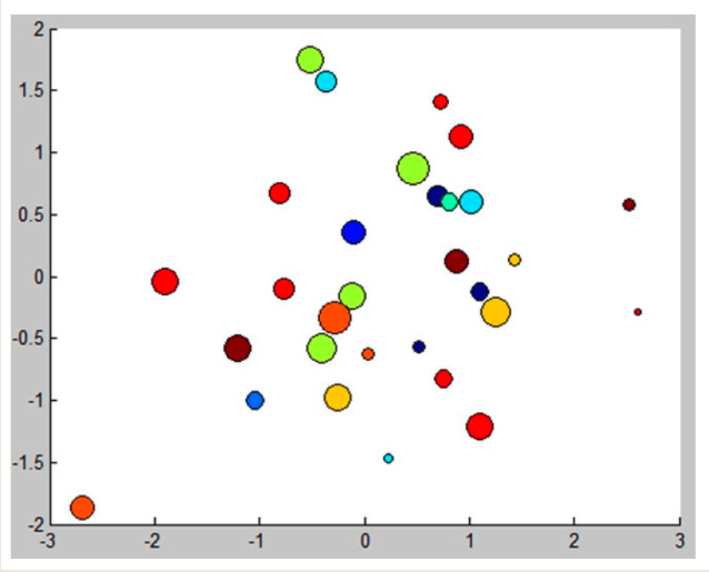
The Bubble Chart allows for the representation of 4-dimensional Efficient Sets by embedding:

• Two objectives on the x and y axes;
• A third objective through bubble size;
• A fourth objective through color.

This makes it possible to interpret four dimensions within a single 2D plot, using visual encodings for the extra information.

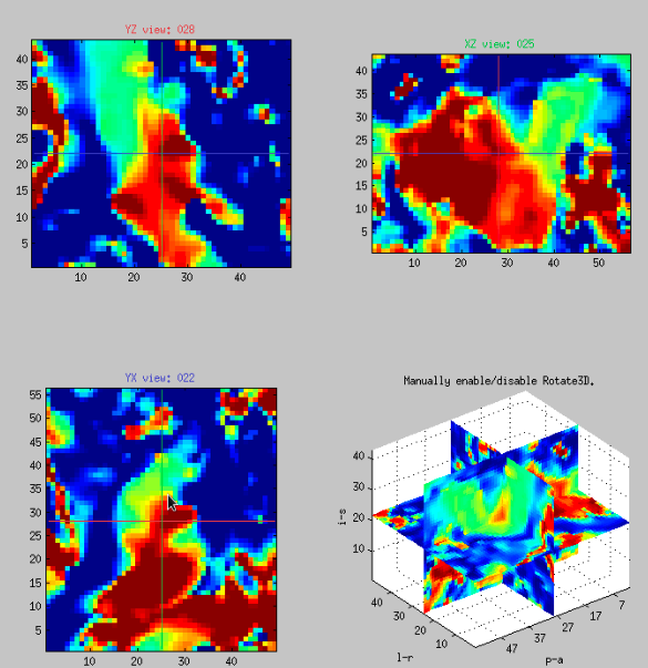
When visualizing 4D data, one approach is to rely on traditional 3D representations and use color encoding or slicing to incorporate a fourth variable. This is appropriate when the fourth variable is sampled on a regular 3D grid, as in volume visualization.

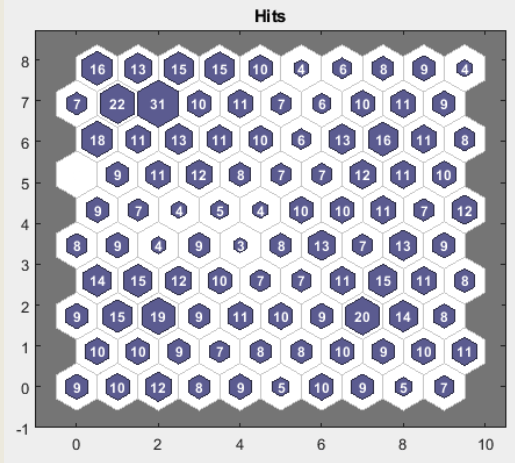
Self-Organizing Maps (SOMs) are unsupervised neural networks that project M-dimensional datasets onto a 2D space while preserving topological properties.

The typical SOM-based visualization involves:

1. Training the SOM with the input data;
2. Assigning each data point to its closest centroid;
3. Counting how many points are associated with each centroid;
4. Coloring each 2D cell proportionally to this count.

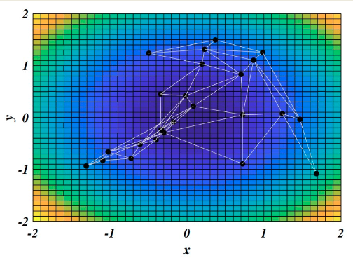
A challenge with classical SOMs (cSOM) is that they tend to fold or self-intersect, distorting the visualization.

To overcome the limitations of classical SOMs, the iSOM (interpretable SOM) was introduced. It avoids folding and preserves the topography of the input data.

Advantages of iSOM include:

• Maintaining continuity and distance relationships;
• Better interpretability;
• Applicability to design space exploration and Efficient Set visualization.

Example: cSOM vs iSOM

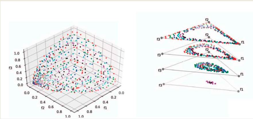
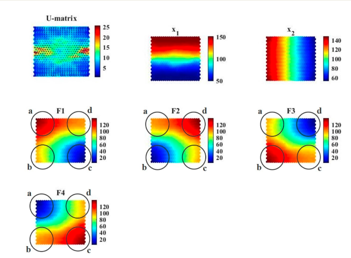
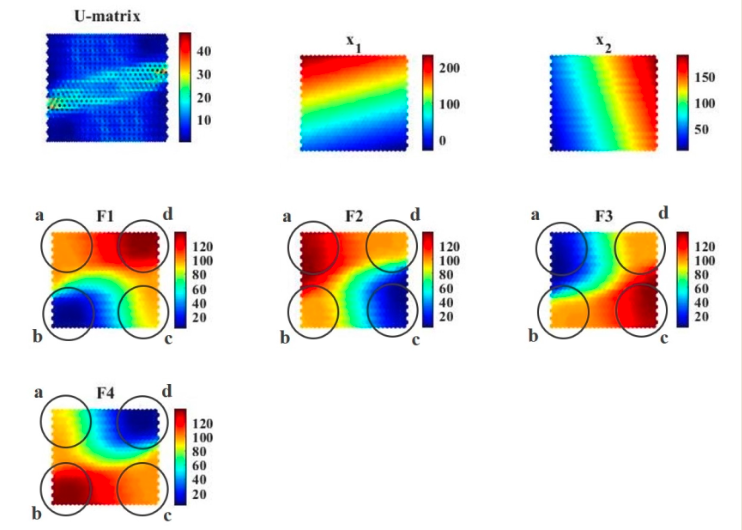
Let’s consider a four-objectives problem with two input variables stated as follows: $$F_1 = \sqrt{(x_1-50)^2+(x_2-50)^2}$$ $$F_2 = \sqrt{(x_1-50)^2+(x_2-150)^2}$$ $$F_3 = \sqrt{(x_1-150)^2+(x_2-50)^2}$$ $$F_4 = \sqrt{(x_1-150)^2+(x_2-150)^2}$$ On the left, cSOM grid in Pareto Space after training, while on the right the iSOM grid.

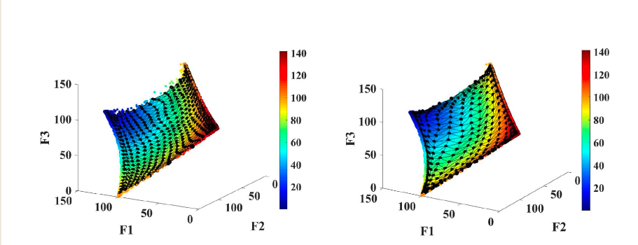
With the cSOM results:

and the iSOM results:

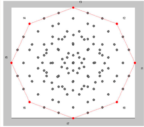
RadViz

RadViz is a radial visualization method based on the idea of spring equilibrium. Each objective is assigned to a vertex of a regular polygon, and each data point is connected to every objective via a virtual spring.

• Points with balanced values across all objectives will appear near the center.
• Points with high values for one objective will be pulled toward the corresponding vertex.

All values must be normalized in $[0, 1]$ for this to work.

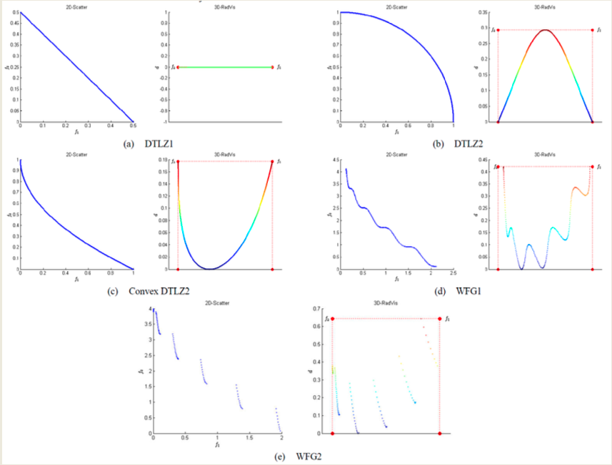
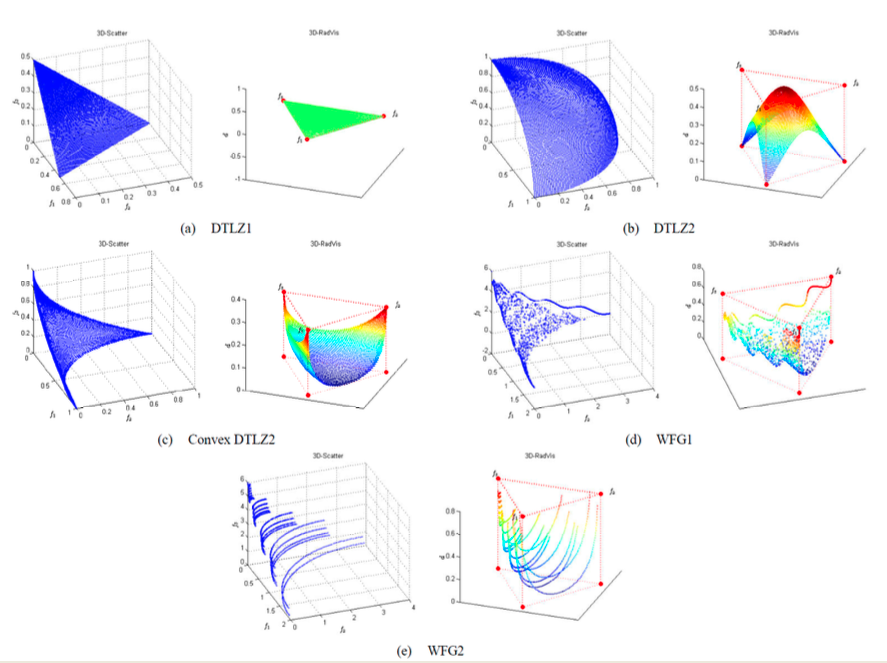
3D-RadViz extends RadViz to three dimensions, enhancing interpretability and preserving the structure of the Efficient Set. The algorithm works as follows:

1. Compute a hyperplane passing through the canonical basis points $[1, 0, …, 0], [0, 1, …, 0], [0, 0, …, 1]$;
2. Calculate the distance $d_i$ of each point from this hyperplane;
3. Project the points onto a 2D RadViz plot;
4. Use the distance $d_i$ to define the elevation of each point in 3D.

This method preserves shape, distribution, and convergence trends of many-objective solution sets.

PaletteVis is a more recent technique aimed at visualizing high-dimensional Pareto fronts while preserving topological consistency. Unlike other techniques, it focuses on accurately maintaining the neighborhood structure among points in the Efficient Set.

This method improves the interpretability and decision-support capabilities in many-objective problems, especially when structure and relationships among solutions are critical.