Reinforcement Learning - Model Free Methods
In many real-world scenarios, it is impractical or impossible to assume full knowledge of the environment’s dynamics, such as the transition probabilities or the reward function. For this reason, model-free reinforcement learning techniques have been developed. These approaches allow an agent to learn from direct interaction with the environment, without requiring an explicit model.
Two primary categories of model-free, sample-based methods for policy evaluation are:
- Monte Carlo (MC) methods
- Temporal Difference (TD) methods
Each of these approaches has distinct characteristics in terms of how they learn and update estimates of the value function.
Monte Carlo Reinforcement Learning
Monte Carlo methods rely on learning from complete episodes of experience. Each episode is a sequence of states, actions, and rewards collected under a fixed policy $\pi$. Learning occurs offline, after the episode has terminated.
Some key characteristics of MC methods:
- Unbiased estimates: MC returns are unbiased estimates of the true value function.
- High variance: Due to their reliance on full episodes and random sampling, MC estimates often exhibit high variance.
Temporal Difference Reinforcement Learning
Temporal Difference methods perform incremental learning from individual transitions, rather than complete episodes. They combine aspects of Monte Carlo methods and dynamic programming.
Key characteristics of TD methods:
- Biased estimates: TD employs bootstrapping, introducing a bias in exchange for faster convergence.
- Low variance: Estimates generally have lower variance compared to MC.
MC Policy Evaluation
Monte Carlo policy evaluation aims to estimate the value function: $$ V_\pi(s) = \mathbb{E}\pi \left[ G_t^T \mid s_t = s \right], $$ where: $$ G_t^T = \sum{k=t}^{T-1} \gamma^{k} , r_{t+k+1}. $$ Episodes are collected by exploring the environment with policy $\pi$. A sequence of samples $\langle S, A, R, S’ \rangle$ is generated, and an episode refers to a complete empirical sequence of such samples. The maximum episode length is denoted by $T$.
Two variants of MC evaluation exist:
- First-encounter MC: Only the first visit to each state in an episode contributes to value updates.
- Every-encounter MC: Every occurrence of each state in the episode contributes to value updates.
The Every-Encounter MC Policy Evaluation Algorithm is the following:
- Initialize:
- $V(s) = 0$ and $N(s) = 0$ for all $s \in \mathcal{S}$.
- $G(s) = 0$ for all $s \in \mathcal{S}$.
- For each episode $e \in \mathcal{E}$:
- For $t = T-1$ to $0$:
- Increment counter: $N(s_t) = N(s_t) + 1$.
- Update return sum: $G(s_t) = G(s_t) + G_t$.
- For $t = T-1$ to $0$:
- Final value estimation:
- $V(s) = \frac{G(s)}{N(s)}$ for each state $s$.
To optimize the algorithm and avoid storing $G(s)$ explicitly, an incremental mean update can be used: $$ \mu_k = \frac{1}{k} \sum_{i=1}^k x_i = \mu_{k-1} + \frac{1}{k} (x_k - \mu_{k-1}). $$ Thus, after each episode: $$ V(s_t) = V(s_t) + \frac{1}{N(s_t)} (G_t - V(s_t)). $$
TD Policy Evaluation
Temporal Difference learning updates the value function after each transition, not after entire episodes. It relies on the following update rule: $$ V(s_t) = V(s_t) + \nu (G_t - V(s_t)), $$ where: $$ G_t = r_{t+1} + \gamma V(s_{t+1}). $$ The TD(0) algorithm thus combines actual rewards with bootstrapped estimates of future values.
Key Properties
- The algorithm proceeds incrementally.
- It does not require episodes to be finite or terminating.
- The initial value function is typically set to $V(s) = 0$ for all states.
- Convergence to optimality is guaranteed when $0 < \nu \ll 1$, though the order of sample processing can affect results.
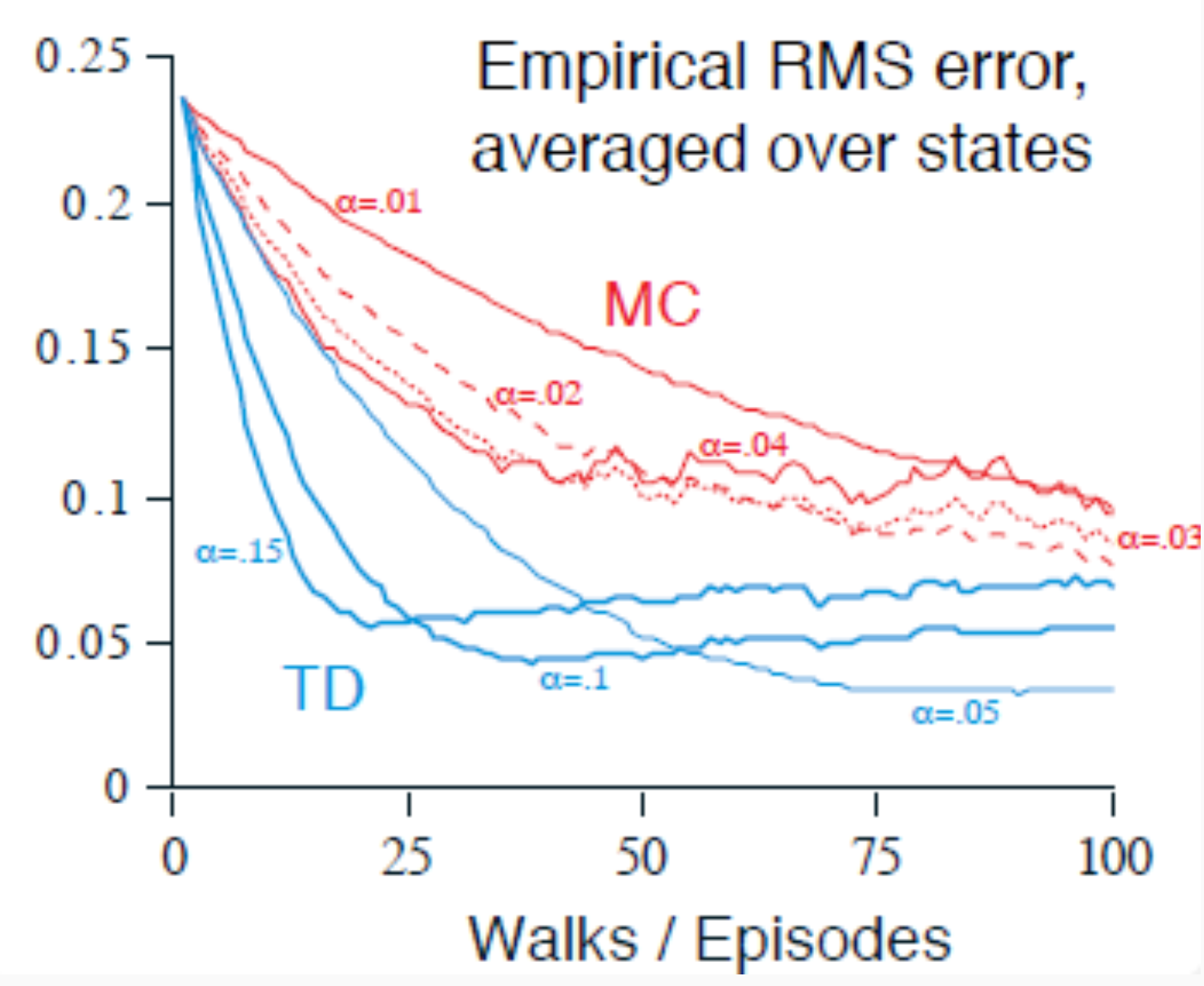
In practice, TD methods generally converge faster than MC methods. The variant described here is known as TD(0), based on the form of $G_t$ used.
Reasoning Example
To better understand the differences between Monte Carlo (MC) and Temporal Difference (TD) methods, consider the example depicted in the following figure:

The possible transitions are as follows:
- From A, the agent always moves to B with probability $1$, receiving a reward $r = 0$.
- From B, the agent transitions to a terminal state according to the following probabilities:
- With $75%$ probability, the agent obtains reward $r = 1$ and terminates the episode.
- With $25%$ probability, the agent obtains reward $r = 0$ and terminates the episode.
Here the observed transitions and rewards:
- A, 0, B, 0
- B, 1
- B, 1
- B, 1
- B, 0
In total, the following transitions were observed:
- From A, a single transition was observed: $A \to B$ with reward $0$.
- From B, $4$ terminal transitions were observed with rewards: $[1, 1, 1, 0]$.
Monte Carlo methods compute the value of a state as the empirical average of the total return observed in episodes starting from that state.
For B: The observed terminal rewards are $[1, 1, 1, 0]$. Thus:$$V(B) = \frac{1 + 1 + 1 + 0}{4} = \frac{3}{4} = 0.75$$
For A: The only observed episode starting from A involved the transition $A \to B$ with reward $0$, followed by the transition from B with reward $0$. Thus:$$V(A) = 0$$ Temporal Difference (TD(0)) methods update the value of a state incrementally, using the bootstrapped estimate of the next state’s value: $$ V(s_t) \leftarrow V(s_t) + \nu \left( r_{t+1} + \gamma V(s_{t+1}) - V(s_t) \right) $$ In the example:
For B: TD will iteratively update $V(B)$ towards the observed expected return. After sufficient updates, $V(B)$ will converge to approximately $0.75$, matching the MC estimate.
For A: Since A always transitions deterministically to B with reward $0$, and assuming $V(B) = 0.75$, the value of A will converge to:$$ V(A) = \gamma \cdot V(B) = 0.99 \times 0.75 = 0.7425 \approx 0.74 $$This is because, when the value function has converged, the value of a state must satisfy the equilibrium condition implied by the TD(0) update rule. In equilibrium, the estimate no longer changes, which means the value of A must already reflect the expected return from moving immediately to B and receiving its value, discounted by $\gamma$. Hence: $$ V(A) = 0 + \gamma \cdot V(B) $$
| State | MC value | TD value |
|---|---|---|
| A | 0 | 0.74 |
| B | 0.75 | 0.75 |
| This example clearly highlights the conceptual differences: |
- MC computes the value of a state as an average over complete episodes.
- TD updates the value incrementally by bootstrapping on current estimates of subsequent states.
In this particular example:
- The value of B converges to the same estimate under both approaches.
- The value of A under TD reflects the discounted value of B, whereas MC remains at $0$ due to the lack of observed positive return in the only sampled episode from A.
This illustrates the strength of TD methods: they can propagate value information even when the full return is not yet observed, making them more suitable for online learning.
MC vs TD in Policy Estimation
Monte Carlo
MC methods aim to minimize the mean squared error between the observed returns and the estimated values: $$ V_\pi = \arg\min_V , \sum_{e=1}^{E} \sum_{t=0}^{T_e-1} (G_t - V(s_t))^2 . $$ However, this process does not respect the Markovian property of the environment.
Temporal Difference
TD(0) methods aim for a maximum likelihood estimation of transitions and rewards: $$ \hat{P}^a_{ss^\prime} = \frac{1}{N(s,a)} \sum_{e=1}^{E} \sum_{t=0}^{T_e-1} \mathbb{1} \left(s_t^{(e)}, a_t^{(e)}, s_{t+1}^{(e)}; s, a, s^\prime \right), $$ $$ \hat{R}^a_{s} = \frac{1}{N(s,a)} \sum_{e=1}^{E} \sum_{t=0}^{T_e-1} \mathbb{1}\left(s_t^{(e)}, a_t^{(e)}; s, a\right) , r_t^{(e)}. $$
This approach explicitly leverages the Markovian nature of the problem.
Summary of Differences
| Aspect | Monte Carlo (MC) | Temporal Difference (TD) |
|---|---|---|
| Learning type | Offline | Online |
| Bootstrapping | No | Yes |
| Bias | No | Yes |
| Variance | High | Low |
| Speed of convergence | Slower | Faster |
| Respect Markov property? | No | Yes |
Noise and Convergence
Both MC and TD approaches must deal with noise in the environment’s rewards and transitions. Their convergence behavior depends heavily on:
- The learning rate $\nu$.
- The degree of variance in returns.
- The order in which samples are processed.
TD typically converges faster, but may introduce bias. MC is unbiased but may require many more samples to achieve reliable estimates.
Model-Free On-Policy Optimization
In reinforcement learning, a central distinction exists between on-policy and off-policy learning:
- On-policy learning aims to evaluate or improve the policy $\pi$ while generating data by following the same policy $\pi$.
- Off-policy learning aims to evaluate or improve the target policy $\pi$ while collecting experience from a different behavior policy $\mu$.
In this section, we focus on model-free on-policy optimization methods, which aim to improve the agent’s behavior directly from its own interactions with the environment, without requiring a model of the environment.
Generalized Policy Iteration (GPI)
A natural idea for on-policy optimization is to follow the Generalized Policy Iteration (GPI) framework:
- Given the current policy $\pi_k$, compute its value function $V_{\pi_k}$.
- Use $V_{\pi_k}$ to improve the policy to $\pi_{k+1}$.
- Repeat the process by setting $k \leftarrow k + 1$.
However, in a model-free setting, this process faces some key challenges:
- The environment dynamics (transition probabilities $P^a_{ss’}$ and rewards $R^a_s$) are unknown.
- The greedy improvement step:$$ \pi_{k+1}(a|s) = \arg\max_{a \in A} \left( R^a_s + P^a_{ss’} V_{\pi_k}(s’) \right) $$cannot be directly implemented without this knowledge. An alternative is to learn an action-value function $Q_{\pi_k}(s, a)$ directly from experience and use it to perform policy improvement:$$ \pi_{k+1}(a|s) = \arg\max_{a \in A} Q_{\pi_k}(s,a) $$This bypasses the need to estimate $P^a_{ss’}$ and $R^a_s$ separately.
Exploration Challenge
A second major issue arises during policy improvement:
- If the initial policy $\pi_0$ is stochastic, the first greedy improvement $\pi_1$ becomes deterministic.
- Without exploration, the agent may converge prematurely to a suboptimal policy.
To ensure continued exploration, the $\varepsilon$-greedy policy is used: $$ \pi_k(a|s) = \begin{cases} \frac{\varepsilon}{m} + (1-\varepsilon) & \text{if } a = \arg\max_{a \in A} Q_{\pi}(s,a) \ \frac{\varepsilon}{m} & \text{otherwise} \end{cases} $$ where:
- $\varepsilon$ controls the degree of exploration.
- $m$ is the number of possible actions in state $s$.
An $\varepsilon$-greedy policy update guarantees that the new policy $\pi_{k+1}$ is at least as good as the current policy $\pi_k$: $$V_{\pi_{k+1}}(s) \geq V_{\pi_k}(s), \quad \forall s \in S$$
Proof Sketch.
The new policy is a weighted combination of exploratory and greedy components. The greedy component ensures that: $$V_{\pi_{k+1}}(s) = \sum_{a \in A} \pi_{k+1}(a | s) Q_{\pi_k}(s,a) = $$ $$= \frac{\epsilon}{m} \sum_{a \in A} Q_{\pi_k}(s,a) + (1-\epsilon) \max_{a \in A} Q_{\pi_k}(s, a) \ge $$ $$= \frac{\epsilon}{m} \sum_{a \in A} Q_{\pi_k}(s,a) + (1-\epsilon) \frac{\pi_k(a|s) - \frac{\epsilon}{m}}{1-\epsilon} Q_{\pi_k}(s, a) = $$ $$= \sum_{a \in A} \pi_{k}(a | s) Q_{\pi_k}(s,a) = $$ while the exploratory component adds an unbiased averaging term that does not degrade performance.
The Bellman optimality equation defines the optimal value function for a deterministic policy. Since $\varepsilon$-greedy policies are stochastic, the following question arises:
Does the algorithm still converge to the optimal policy?
The GLIE Property
$\displaystyle \lim_{k \to \infty} N_k(s,a) = \infty$ Every state-action pair is visited infinitely often.
$\displaystyle \lim_{k \to \infty} \pi_k(a|s) = \mathbb{1}\left(a; \arg\max_{a’ \in A} Q_k(s,a’) \right)$ The policy converges to the greedy policy.
$\varepsilon_k \in O\left( \frac{1}{k} \right)$ The exploration parameter decays appropriately to zero.
If GLIE holds, the policy improvement process will converge to the optimal policy.
On-Policy Optimization Algorithms
Several on-policy optimization algorithms satisfy the GLIE property. They rely on different update mechanisms for the action-value function $Q(s,a)$.
Monte Carlo Optimization Iteration
Monte Carlo-based policy optimization proceeds as follows:
- For each $(s_t, a_t)$ observed in an episode: $$ N(s_t,a_t) \leftarrow N(s_t,a_t) + 1 $$ $$ Q(s_t,a_t) \leftarrow Q(s_t,a_t) + \frac{1}{N(s_t,a_t)} \left( G_t - Q(s_t,a_t) \right) $$
- Update exploration parameter: $$ \varepsilon \leftarrow \frac{1}{k} $$
- Update the policy: $$ \pi_{k+1} \leftarrow \varepsilon\text{-greedy}(Q) $$
Temporal Difference (TD) Optimization
TD-based optimization follows the same philosophy as TD evaluation but now focuses on updating $Q(s,a)$.
SARSA
SARSA learns from on-policy samples of the form $(S, A, R, S’, A’)$. Update rule: $$ Q(s,a) \leftarrow Q(s,a) + \nu \left( r + \gamma Q(s’,a’) - Q(s,a) \right) $$ To guarantee convergence, the learning rate $\nu_t$ must satisfy the Robbins-Monro condition: $$ \sum_{t=1}^{\infty} \nu_t = \infty \quad \text{and} \quad \sum_{t=1}^{\infty} \nu_t^2 < \infty $$
Expected SARSA
Expected SARSA uses the expectation over the next action distribution: $$ Q(s,a) \leftarrow Q(s,a) + \nu \left( r + \gamma \sum_{a’ \in A} \pi(a’|s’) Q(s’,a’) - Q(s,a) \right) $$ Expected SARSA is often more stable, but it becomes computationally challenging when the action space is large, since the expectation requires summing over all actions.
Model-Free Off-Policy Optimization
Off-policy learning provides important flexibility and efficiency advantages in reinforcement learning. In particular, it enables:
- Learning from imitation (leveraging expert demonstrations).
- Re-using experience generated by older policies.
- Learning an optimal policy while following an exploratory one.
- Learning multiple policies while interacting with the environment under a single behavior policy.
- Avoiding real-world re-testing, which can be expensive or infeasible.
The key mathematical tool that enables off-policy learning is importance sampling.
$$\mathbb{E}{x \sim P}[f(x)] = \int_x P(x) f(x) , dx$$ This can be rewritten as: $$= \int_x Q(x) \frac{P(x)}{Q(x)} f(x) , dx = \mathbb{E}{x \sim Q} \left[ \frac{P(x)}{Q(x)} f(x) \right]$$ Thus, one can approximate expectations under $P$ by re-weighting samples from $Q$.
Off-Policy Optimization Algorithms
Monte Carlo Optimization
In off-policy Monte Carlo (MC) optimization, two notions of return are defined:
- $G_t^\mu$: return observed under the behavior policy $\mu$.
- $G_t^\pi$: return corrected to approximate what would have been obtained under the target policy $\pi$.
The importance sampling correction yields: $$ G_t^\pi = \prod_{i=t}^T \frac{\pi(a_i | s_i)}{\mu(a_i | s_i)} G_t^\mu $$ The corresponding update rule is: $$ Q(s_t, a_t) \leftarrow Q(s_t, a_t) + \nu \left( G_t^\pi - Q(s_t, a_t) \right) $$ Practical Consideration
- Importance sampling can introduce high variance.
- For this reason, the behavior policy $\mu$ should be as close as possible to the target policy $\pi$.
Temporal Difference (TD) Optimization
Off-policy TD learning requires only one correction factor per step, thus reducing variance.
Update rule: $$ Q(s, a) \leftarrow Q(s, a) + \nu , \left[ \frac{\pi(a|s)}{\mu(a|s)} \left( r_{t+1} + \gamma Q(s’, a’) \right) - Q(s, a) \right] $$
- Only a single importance sampling correction $\frac{\pi(a|s)}{\mu(a|s)}$ is applied at each step.
Q-Learning
Q-learning can be viewed as a special case of off-policy TD optimization:
- The target policy $\pi$ is chosen to be greedy: $$ \pi(s) = \arg\max_{a \in A} Q(s,a) $$
- The behavior policy $\mu$ is chosen to be $\varepsilon$-greedy:$$\mu(s) = \varepsilon\text{-greedy}(Q(s,a))$$ In this setting, no explicit importance sampling is used.
Update rule: $$ Q(s, a) \leftarrow Q(s_t, a_t) + \nu \left( r_{t+1}^\mu + \gamma Q(s_{t+1}, a_{t+1}^\pi) - Q(s_t, a_t) \right) $$
- $r_{t+1}^\mu$ is obtained by acting under $\mu$.
- $a_{t+1}^\pi$ is chosen greedily by $\pi$.
Simplification of the learning target can be: $$ r_{t+1}^\mu + \gamma Q(s_{t+1}, a_{t+1}^\pi) = r_{t+1}^\mu + \gamma , Q \left( s_{t+1}, \arg\max_{a’ \in A} Q(s_{t+1}, a’) \right )= $$ $$ = r_{t+1}^\mu + \gamma \max_{a’ \in A} Q(s_{t+1}, a’) $$ Q($\lambda$) is a straightforward generalization of Q-learning with eligibility traces.
Beyond TD(0): TD(n) and TD(λ)
Both TD(n) and TD(λ) extend TD(0) by using longer or averaged returns, leading to faster and more accurate learning.
TD(n)
In TD(n), the value update uses an $n$-step lookahead return: $$ V(s_t) = V(s_t) + \nu \left( G_t^{(n)} - V(s_t) \right) $$ where: $$ G_t^{(n)} = \sum_{k=0}^{n} \gamma^k r_{t+k+1} + \gamma^{n+1} V(s_{t+n+1}) $$
TD(λ)
TD(λ) averages multiple $n$-step returns with exponentially decaying weights:
$$ V(s_t) = V(s_t) + \nu \left( G_t^{(\lambda)} - V(s_t) \right) $$
where:
$$ G_t^{(\lambda)} = (1 - \lambda) \sum_{n=1}^{N} \lambda^{n-1} G_t^{(n)} $$
- $N$ can be as large as needed.
- $\lambda \in (0,1)$.
- The normalization ensures:
$$ \sum_{n=1}^{\infty} (1 - \lambda) \lambda^{n-1} = 1 $$
Note:
- Both TD(n) and TD(λ) are typically offline methods, as they require access to complete episodes.
Eligibility Traces and Backward TD(λ)
Backward TD(λ) provides an efficient online implementation of TD(λ) using eligibility traces.
Eligibility Function
An eligibility function $E: S \to \mathbb{R}^+$ tracks how much recently visited states contribute to learning updates:
$$ E_0(s) = 0 $$
$$ E_t(s) = \gamma \lambda E_{t-1}(s) + \mathbb{1}(s_t; s) $$
Backward TD(λ) Update Rule
$$ V(S) = V(S) + \nu , \delta_t , E_t(S) $$
where the TD error $\delta_t$ is:
$$ \delta_t = r_{t+1} + \gamma V(s_{t+1}) - V(s_t) $$
Example Parameters
With $\gamma = 1$, $\lambda = 0.5$, $\nu = 0.99$, and a constant reward $r_{t+1} = 1$, we can carefully observe how the backward TD(λ) algorithm updates the value function $V(S)$ over successive transitions between states. At each step, the eligibility traces accumulate evidence of recent state visits, effectively allowing the TD error $\delta$ to influence not just the current state but a decaying trail of previously visited states. This is precisely the role of the eligibility function $E(S)$, which decays geometrically over time unless a state is revisited, in which case its eligibility is incremented directly.
The updates proceed as follows. Initially, all state values $V(S)$ are zero. After the first transition from $s_1$ to $s_2$, $s_1$’s eligibility trace leads to its value being increased proportionally to $\delta = 1$. As we move from $s_2$ to $s_3$, $s_2$’s eligibility takes over, and similarly, its value begins to grow. The eligibility traces from $s_1$ and $s_2$ persist but decay via the factor $\gamma\lambda = 0.5$, allowing prior states to retain a diminishing influence on updates. This process continues as the system loops back from $s_3$ to $s_1$, where cumulative eligibility traces now include contributions from multiple previous visits. The eligibility for $s_3$ is maximized upon visiting it, while those of $s_1$ and $s_2$ have decayed but still play a role.
The final step shows the transition from $s_1$ to $s_4$, with the accumulated eligibility traces resulting in a more complex update: some states receive negative corrections due to the sign of $\delta$. This reflects the dynamics of TD(λ), where overestimation from previous steps can be counteracted when future evidence does not support it. The negative $\delta$ observed in the final step illustrates this adjustment process.
Overall, this example demonstrates how TD(λ), through the mechanism of eligibility traces, propagates reward information not only forward through successive states but also backward to past states in proportion to their recency and frequency of visitation. The parameters used ($\lambda$, $\gamma$, $\nu$) control how quickly this information spreads and how sharply eligibility fades, balancing stability and speed of learning.
$$ \begin{array}{cccc} V(S) & & E(S) & \delta & V(S) \ \left[\begin{array}{c} 0.00 \ 0.00 \ 0.00 \ 0.00 \end{array}\right] & s_1 \rightarrow s_2 & \left[\begin{array}{c} 1.00 \ 0.00 \ 0.00 \ 0.00 \end{array}\right] & 1.00 & \left[\begin{array}{c} 0.99 \ 0.00 \ 0.00 \ 0.00 \end{array}\right] \ \ \left[\begin{array}{c} 0.99 \ 0.00 \ 0.00 \ 0.00 \end{array}\right] & s_2 \rightarrow s_3 & \left[\begin{array}{c} 0.50 \ 1.00 \ 0.00 \ 0.00 \end{array}\right] & 1.00 & \left[\begin{array}{c} 1.48 \ 0.99 \ 0.00 \ 0.00 \end{array}\right] \ \ \left[\begin{array}{c} 1.48 \ 0.99 \ 0.00 \ 0.00 \end{array}\right] & s_3 \rightarrow s_1 & \left[\begin{array}{c} 0.25 \ 0.50 \ 1.00 \ 0.00 \end{array}\right] & 2.48 & \left[\begin{array}{c} 2.09 \ 1.60 \ 0.61 \ 0.00 \end{array}\right] \ \ \left[\begin{array}{c} 2.09 \ 1.60 \ 0.61 \ 0.00 \end{array}\right] & s_1 \rightarrow s_4 & \left[\begin{array}{c} 1.13 \ 0.25 \ 0.50 \ 0.00 \end{array}\right] & -1.09 & \left[\begin{array}{c} 0.87 \ 1.33 \ 0.09 \ 0.00 \end{array}\right] \ \end{array} $$
SARSA(n), SARSA(λ), and Variants
SARSA(n)
SARSA(n) extends SARSA by using n-step returns:
$$ Q(s, a) \leftarrow Q(s, a) + \nu \left( r + \gamma , Q_t^{(n)} - Q(s,a) \right) $$
where:
$$ Q_t^{(n)} = \sum_{k=0}^n \gamma^k r_{t+k+1} + \gamma^{n+1} Q(s_{t+n+1}, a_{t+n+1}) $$
SARSA(λ)
SARSA(λ) averages $n$-step returns similarly to TD(λ):
$$ Q(s, a) \leftarrow Q(s, a) + \nu \left( r + \gamma Q_t^{(\lambda)} - Q(s,a) \right) $$
where:
$$ Q_t^{(\lambda)} = (1 - \lambda) \sum_{n=1}^{N} \lambda^{n-1} Q_t^{(n)} $$
$$ \sum_{n=1}^{\infty} (1 - \lambda) \lambda^{n-1} = 1 $$
Backward SARSA(λ)
Backward SARSA(λ) efficiently implements SARSA(λ) online using eligibility traces:
$$ Q(S, A) \leftarrow Q(S, A) + \nu , \delta_t , E_t(S,A) $$
with:
$$ \delta_t = r_{t+1} + \gamma , Q(s_{t+1}, a_{t+1}) - Q(s_t, a_t) $$
Eligibility trace update:
$$ E_t(s,a) = \gamma , \lambda , E_{t-1}(s,a) + \mathbb{1}(s_t, a_t; s, a) $$
$$ E_0(s,a) = 0 $$