Mixed Pareto-Lexicographic Optimization
In many real-world scenarios, not all objectives are equally important. Some goals must be achieved with higher priority, while others may be considered only if the most important ones are satisfied or optimized. This intuition leads to the study of Mixed Pareto-Lexicographic (MPL) optimization problems, which aim to combine the strengths of lexicographic and Pareto-based approaches within multi-objective optimization.
Pure Lexicographic Optimization
A lexicographic multi-objective optimization problem assumes a strict hierarchy among objectives. The formal expression is: $$ \text{Lexmin } f_1(x), f_2(x), \dots, f_M(x) \quad \text{subject to } x \in \Omega $$ This formulation dictates that minimizing $f_1(x)$ is infinitely more important than minimizing $f_2(x)$, which in turn is more important than minimizing $f_3(x)$, and so on. The optimizer considers each function in strict order: only if two solutions have the same value for the first objective, their second objective is evaluated, and so forth.
To understand how lexicographic ordering works, consider two vectors of equal length. If we compare $[3, 4]$ with $[2, 8]$ under lexicographic ordering, the result is false since $3 > 2$. However, comparing $[3, 4]$ with $[3, 7]$ returns true, as the first elements are equal and $4 < 7$. The lexicographic rule thus follows the logic of dictionaries: comparisons are made element by element, in order.
Introducing the Grossone Methodology
The rigid structure of pure lexicographic optimization led researchers to explore more flexible formulations. One of the tools used to represent infinite priority relations is the Grossone Methodology, proposed by Yaroslav D. Sergeyev in 2003. This methodology introduces a symbolic infinite number, denoted by $①$, which serves as an analogue of Benci’s $\alpha$ in the Alpha-Theory. Its reciprocal, $①^{-1}$, represents an infinitesimal quantity, similar to Benci’s $\eta$.
By using Grossone, it becomes possible to express optimization problems in which certain objectives dominate others with an infinite or infinitesimal weight, thereby encoding priorities more effectively in numerical terms.
Alpha-Theory is a mathematical framework introduced by Vieri Benci and collaborators to rigorously handle infinitesimal and infinite numbers within analysis and computation.
In this theory:
- $\alpha$ (alpha) represents a fixed infinite number, which can be used to define extended numerical fields that include both infinite and infinitesimal elements.
- $\eta$ (eta) is its reciprocal, i.e., $\eta = \frac{1}{\alpha}$, and it represents a positive infinitesimal, which is smaller than any positive real number but still greater than zero.
Alpha-Theory enables the formal manipulation of such numbers, offering an alternative to nonstandard analysis. It has been used to define new types of real number extensions, including PANs (Polynomial Algorithmic Numbers), which are used in optimization to model objectives that combine priorities across multiple scales (like infinite and infinitesimal).
Mixed Pareto-Lexicographic Optimization: The Case of Priority Chains
One of the most studied formulations in the MPL framework is the Priority Chains (PC) approach. In this model, each objective can be expressed as a combination of sub-objectives, ordered by priority and weighted using powers of the infinitesimal $①^{-1}$. The general expression becomes: $$ \min \begin{bmatrix} \text{lexmin} \left( f_1^{(1)}(x), f_1^{(2)}(x), \dots, f_1^{(p_1)}(x) \right) \ \text{lexmin} \left( f_2^{(1)}(x), f_2^{(2)}(x), \dots, f_2^{(p_2)}(x) \right) \ \vdots \ \text{lexmin} \left( f_m^{(1)}(x), f_m^{(2)}(x), \dots, f_m^{(p_m)}(x) \right) \end{bmatrix} \Rightarrow $$ $$\Rightarrow \min \begin{bmatrix} f_1^{(1)}(x) + ①^{-1} f_1^{(2)}(x) + \dots + ①^{-(p_1 - 1)} f_1^{(p_1)}(x) \ f_2^{(1)}(x) + ①^{-1} f_2^{(2)}(x) + \dots + ①^{-(p_2 - 1)} f_2^{(p_2)}(x) \ \vdots \ f_m^{(1)}(x) + ①^{-1} f_m^{(2)}(x) + \dots + ①^{-(p_m - 1)} f_m^{(p_m)}(x) \end{bmatrix} \triangleq \min \begin{bmatrix} \underline{f_1}(x) \ \underline{f_2}(x) \ \vdots \ \underline{f_m}(x) \end{bmatrix} $$ where each $$ \underline{f_i}(x) = f_i^{(1)}(x) + ①^{-1} f_i^{(2)}(x) + ①^{-2} f_i^{(3)}(x) + \dots $$ is a gross scalar (a PAN - Polynomial Algorithmic Number - scalar value in the Alpha Theory Terminology).
This allows defining a scalar quantity that encodes the entire chain of objectives, ensuring that improvements in the highest-priority sub-objectives always dominate changes in the lower-priority ones.
To solve such problems, a new form of dominance, called PC-dominance, must be introduced. This relation extends the traditional Pareto dominance by incorporating infinitesimal coefficients to represent sub-objective influence.
Given two solutions $A$ and $B$, $A$ dominates $B$ (written $A \preceq B$) if the following relation holds:
$$ A \preceq B \iff \begin{cases} \underline{f_i}(x_A) \leq \underline{f_i}(x_B) & \forall i = 1, \dots, m \ \exists j \text{ such that } \underline{f_j}(x_A) < \underline{f_j}(x_B) \end{cases} $$
A concrete and instructive example of the Priority Chains formulation is given by the 0-1 Knapsack problem, adapted to a multi-objective context. In its MPL version, the objective functions are structured into two chains of priorities. The first chain, denoted as $f_1(x)$, represents the total profit obtained by selecting a subset of items. This profit is composed of two components: a primary component corresponding to the overall monetary gain ($V_1^{(1)}$), and a secondary component that quantifies the portion of profit derived from investments in renewable energy sources ($V_1^{(2)}$). The second chain, denoted as $f_2(x)$, represents the risk associated with the investment choices. Here too, the function is split into two components: the primary component accounts for the general risk of the selected items ($V_2^{(1)}$), while the secondary component specifically measures the risk associated to non-governmental bonds ($V_2^{(2)}$).
This structure makes the problem suitable for a mixed Pareto-Lexicographic treatment. Thanks to the Grossone-based reformulation, the two chains are encoded numerically using infinitesimal weights: the primary objectives dominate the optimization process, while the secondary ones are considered only when solutions are equivalent at the higher priority level. The capacity constraint of the knapsack is still respected in the standard way, by ensuring that the total weight of selected items does not exceed a fixed budget.
There are three main ways to formulate the knapsack problem depending on how multiple objectives are handled.
In the classical formulation, the problem involves a single objective: maximizing the total profit. Each item $i$ is associated with a profit $v_i$ and a weight $w_i$. The objective is to select a subset of items such that the total profit $Vx = \sum_i v_i x_i$ is maximized, under the constraint that the total weight $Wx = \sum_i w_i x_i$ does not exceed the knapsack capacity $C$. The decision variables $x_i$ are binary and indicate whether item $i$ is included in the knapsack or not: $$ \max Vx \quad \text{s.t. } Wx \leq C, \quad x_i \in {0,1} $$ In the pure Paretian formulation, the problem is extended to include two objectives, for instance total profit $V_1x$ and an additional measure like renewable-sourced profit $V_2x$. The optimizer seeks solutions that are not dominated in the Pareto sense, balancing both objectives under the same weight constraint: $$ \max (V_1x, V_2x) \quad \text{s.t. } Wx \leq C, \quad x_i \in {0,1} $$ In the pure lexicographic formulation, the two objectives are no longer considered equally important. Instead, $V_1x$ is given absolute priority over $V_2x$. This is formalized using lexicographic maximization, where $V_2x$ is considered only when two solutions have equal values for $V_1x$: $$ \text{lex max} (V_1x, V_2x) \quad \text{s.t. } Wx \leq C, \quad x_i \in {0,1} $$ Using the Grossone-based numerical formulation, the lexicographic problem can also be written as a single objective where $V_2x$ is multiplied by the infinitesimal $①^{-1}$, preserving the dominance of $V_1x$ while allowing $V_2x$ to influence tie-breaking: $$ \max V_1x + V_2x \cdot ①^{-1} \quad \text{s.t. } Wx \leq C, \quad x_i \in {0,1} $$ This final formulation is particularly useful in evolutionary algorithms, where it simplifies the implementation of lexicographic priority while remaining fully numeric.
Algorithms
To solve such problems efficiently, classical multi-objective evolutionary algorithms are extended. In particular, both NSGA-II and MOEA/D have been adapted to handle priority chains by incorporating a new dominance relation, the PC-dominance. The resulting algorithms, namely PC-NSGA-II and PC-MOEA/D, modify the non-dominated sorting and crowding distance computations to take the priority structure into account, ensuring that higher-priority components always drive the selection process.
The PC-NSGA-II algorithm extends the classical NSGA-II to deal with Priority Chains. The key modifications include a new non-dominated sorting method based on gross-scalars, and a modified crowding distance function that also operates on gross-scalar values.
Procedure: PC_NSGA_II
$R_t \leftarrow P_t \cup Q_t$
/* Fast non-dominated sort with gross-scalar objectives */
$F \leftarrow \text{PC_fast_nondominated_sort}(R_t, 0)$
$P_{t+1} \leftarrow \emptyset$
$i \leftarrow 1$
while $|P_{t+1}| + |F_i| \leq N$ do
/* Crowding distance with gross-scalars */
$\text{PC_crowding_distance_assignment}(F_i)$
$P_{t+1} \leftarrow P_{t+1} \cup F_i$
$i \leftarrow i + 1$
end while
/* Sort by PC_crowded_comparison_operator */
$\text{sort}(F_i, \preceq_n)$
$P_{t+1} \leftarrow P_{t+1} \cup F_i[1 : (N - |P_{t+1}|)]$
$Q_{t+1} \leftarrow \text{make_new_pop}(P_{t+1})$
$t \leftarrow t + 1$
The PC-fast-nondominated-sort procedure is adapted to compare solutions using the PC-dominance relation. For each individual, it tracks the set of solutions it dominates and the number of solutions dominating it. Individuals not dominated by any other are assigned to the first front, and the process repeats iteratively.
Procedure: PC_fast_nondominated_sort(P)
for all $p \in P$ do
$S_p \leftarrow \emptyset$
$n_p \leftarrow 0$
for all $q \in P$ do
if $p \preceq q$ then
$S_p \leftarrow S_p \cup {q}$
else if $q \preceq p$ then
$n_p \leftarrow n_p + 1$
if $n_p = 0$ then
$p_{\text{rank}} \leftarrow 1$
$F_1 \leftarrow F_1 \cup {p}$
$i \leftarrow 1$
while $F_i \neq \emptyset$ do
$Q \leftarrow \emptyset$
for all $p \in F_i$ do
for all $q \in S_p$ do
$n_q \leftarrow n_q - 1$
if $n_q = 0$ then
$q_{\text{rank}} \leftarrow i + 1$
$Q \leftarrow Q \cup {q}$
$i \leftarrow i + 1$
$F_i \leftarrow Q$
The PC-crowding-distance-assignment function is responsible for maintaining diversity within a Pareto front. It operates similarly to the classical version, but the distance values are treated as gross-scalars. Boundary solutions receive the maximum crowding value (Grossone, $①$).
Procedure: PC_crowding_distance_assignment(F)
$n \leftarrow |F|$
for all $i \in F$ do
$F[i]_{\text{dist}} \leftarrow 0$
for $j = 1 \dots m$ do
$F \leftarrow \text{sort}(F, f_j)$
$F[1]{\text{dist}} = F[n]{\text{dist}} = ①$
for $i = 2 \dots (n - 1)$ do
/* the PC_crowding_distance is a gross-scalar */
$F[i]{\text{dist}} = F[i]{\text{dist}} + \dfrac{f_j(F[i+1]) - f_j(F[i-1])}{f_j^{\max} - f_j^{\min}}$
The PC-MOEA/D algorithm is an extension of the decomposition-based MOEA/D framework adapted to Priority Chains. Each subproblem is associated with a weight vector and uses gross-scalar dominance to update its population. The external population is also updated using PC-specific dominance checks.
Procedure: PC_MOEA/D
$EP \leftarrow \emptyset$
for $i = 1 \dots N$ do
$\lambda_i^1, \dots, \lambda_i^T \leftarrow \text{find_closest_weights}(\lambda_i, T)$
$B_i \leftarrow {i_1, \dots, i_T}$
$x^1, \dots, x^N \leftarrow \text{initialize_population}(N)$
$FV^i \leftarrow F(x^i)$
$\mathbf{z}_1, \dots, \mathbf{z}_m \leftarrow \text{initialize_ref_point}(m)$
while stop_criteria() = False do
for $i = 1 \dots N$ do
$k, l \leftarrow \text{rand}(B_i, 2)$
$y \leftarrow \text{make_new_sol}(x^k, x^l)$
$y’ \leftarrow \text{mutate}(y)$
for $j = 1 \dots m$ do
if $z_j < f_j(y’)$ then
$z_j \leftarrow f_j(y’)$
for all $j \in B_i$ do
if $g^{te}(y’ | \lambda^j, z) \leq g^{te}(x^j | \lambda^j, z)$ then
$x^j \leftarrow y’$
$FV^j \leftarrow F(y’)$
$DD \leftarrow \text{PC_find_dominated_sol}(EP, F(y’))$
$DG \leftarrow \text{PC_find_dominating_sol}(EP, F(y’))$
$EP \leftarrow EP \setminus DD$
if $DG = \emptyset$ then
$EP \leftarrow EP \cup F(y’)$
The Priority Levels Approach
Another relevant formulation within the MPL framework is the Priority Levels (PL) approach. While priority chains encode objective dependencies sequentially, the PL model groups objectives into levels of equal importance, where each level has precedence over the next. $$ \text{lexmin} \left[ \min \begin{pmatrix} f_1^{(1)}(\mathbf{x}) \ f_2^{(1)}(\mathbf{x}) \ \vdots \ f_{m_1}^{(1)}(\mathbf{x}) \end{pmatrix}, \min \begin{pmatrix} f_1^{(2)}(\mathbf{x}) \ f_2^{(2)}(\mathbf{x}) \ \vdots \ f_{m_2}^{(2)}(\mathbf{x}) \end{pmatrix}, \dots, \min \begin{pmatrix} f_1^{(p)}(\mathbf{x}) \ f_2^{(p)}(\mathbf{x}) \ \vdots \ f_{m_p}^{(p)}(\mathbf{x}) \end{pmatrix} \right] $$ Thanks again to the Grossone Methodology, this model can be rewritten as: $$ \min \left[ \begin{pmatrix} f_1^{(1)}(\mathbf{x}) \ f_2^{(1)}(\mathbf{x}) \ \vdots \ f_{m_1}^{(1)}(\mathbf{x}) \end{pmatrix}
- ①^{-1} \begin{pmatrix} f_1^{(2)}(\mathbf{x}) \ f_2^{(2)}(\mathbf{x}) \ \vdots \ f_{m_2}^{(2)}(\mathbf{x}) \end{pmatrix}
- \dots + ①^{1-p} \begin{pmatrix} f_1^{(p)}(\mathbf{x}) \ f_2^{(p)}(\mathbf{x}) \ \vdots \ f_{m_p}^{(p)}(\mathbf{x}) \end{pmatrix} \right] $$ $$ f(x) = \text{Level}_1(x) + ①^{-1} \cdot \text{Level}_2(x) + ①^{-2} \cdot \text{Level}_3(x) + \dots $$ However, this formulation requires a novel definition of dominance, referred to as PL-dominance. A naïve extension of PC-dominance to PL does not work, as it fails to preserve transitivity—an essential property for evolutionary algorithms. Indeed, such a definition would claim:
“Given two solutions $A$ and $B$, $A$ is said to PL-dominate $B$ if there exists a priority level $i$ such that $A$ Pareto-dominates $B$ on the objectives of priority level $i$, and $A$ and $B$ are non-dominated at each priority level higher than $i$.”
However, this approach leads to inconsistencies. Consider the following example: $$ A = \binom{2}{5} + ①^{-1} \binom{2}{2}, \quad B = \binom{4}{3} + ①^{-1} \binom{7}{6}, \quad C = \binom{1}{4} + ①^{-1} \binom{9}{8} $$
There exists a dominance loop:
- $A$ PL-dominates $B$ because, although they are non-dominated at the primary level, $A$ performs better than $B$ on the secondary objectives.
- $B$ PL-dominates $C$ for the same reason.
- $C$ PL-dominates $A$ because it does better on the primary objectives.
This circular dominance relation highlights that the naïve definition does not preserve transitivity, thereby motivating the need for a more robust and well-founded dominance relation in PL contexts.
Given two solutions $A$ and $B$, belonging to the subfronts $F_i$ and $F_j$ respectively,
$A$ PL-dominates $B$ if and only if $i < j$:
$$ A \prec^* B \iff i < j $$
It is worth noting the a posteriori nature of this definition: it is not always possible to tell whether two elements are dominated or not before assigning a fitness rank to the whole population.
In other words, the non-dominance relation is not just a function of two arguments (solutions),
but has a global dependency on all the other individuals.
With this new definition in place, the classical fast non-dominated sorting procedure used in NSGA-II is extended to PL_Fast_NonDominated_Sort, which is able to assign both a rank (or front) and a sub-rank (within each level). This makes it possible to generalize NSGA-II into PL-NSGA-II, which is capable of solving many-objective problems involving structured priority levels.
The sorting process is implemented recursively. For each level of priority, the algorithm identifies the set of non-dominated fronts using a specialized subroutine that operates within that level. Once fronts are identified at a level, the algorithm descends recursively to sort solutions at the next level, conditioned on the structure obtained so far.
Procedure: PL_FAST_NONDOMINATED_SORT(P, lvl)
/* This function is recursive */
if $lvl < \text{min_lvl}$ then return
/* The first iteration also initializes all ranks to 0 */
if $lvl == 0$ then
for all $p \in P$ do
$p_{\text{rank}} = 0$
/* Ranking within the priority level to determine subfronts */
$F^{(lvl)} = \text{fast_nondom_sort_in_level}(P, lvl)$
/* Repeat for every subfront found /
for all $F_i \in F^{(lvl)}$ do
/ In the next priority level */
$F_i = \text{PL_fast_nondominated_sort}(F_i, lvl - 1)$
The function FAST_NONDOM_SORT_IN_LEVEL is a modified version of fast non-dominated sorting applied within a single priority level. It assigns a sub-rank using the dominance relation defined at that level. Note that the comparison operator here is priority-level-aware, and thus the sorting reflects the structure imposed by the levels.
Procedure: FAST_NONDOM_SORT_IN_LEVEL(P, lvl)
for all $p \in P$ do
$S_p \leftarrow \emptyset$
$n_p \leftarrow 0$
for all $q \in P$ do
/* non-dominance at specified priority level /
if $p \prec^{lvl} q$ then
$S_p \leftarrow S_p \cup {q}$
else if $q \prec^{lvl} p$ then
$n_p \leftarrow n_p + 1$
if $n_p == 0$ then
/ First subfront within $P$ */
$p_{\text{rank}} = p_{\text{rank}} + ①^{lvl}$
$F_{①^{lvl}} = F_{①^{lvl}} \cup {p}$
$i \leftarrow ①^{lvl}$
while $F_i \neq \emptyset$ do
$Q \leftarrow \emptyset$
for all $p \in F_i$ do
for all $q \in S_p$ do
$n_q \leftarrow n_q - 1$
if $n_q == 0$ then
/* $q$ belongs to the $i$-th subfront */
$q_{\text{rank}} = q_{\text{rank}} + i + ①^{lvl}$
$Q \leftarrow Q \cup {q}$
$i = i + ①^{lvl}$
$F_i = Q$
To maintain diversity, the crowding distance must also be adapted to respect the structure of the priority levels. The distance is now computed by summing scaled components from each level, taking into account their corresponding infinitesimal weights. Solutions at the boundaries receive $+\infty$ as usual.
Procedure: PL_CROWDING_DIST_ASSIGNMENT(F)
$n \leftarrow |F|$
for all $i \in F$ do
$F[i]_{\text{dist}} \leftarrow 0$
/* For each level of priority $q$; $p$ is the index of the last level /
for $q = 1 \dots p$ do
for $j = 1 \dots m_q$ do
$F \leftarrow \text{sort}(F, f_j^{(q)})$
/ +Inf means “full-scale” (IEEE 754 standard) /
$F[1]{\text{dist}} += +\infty \cdot ①^{1 - q}$
$F[n]{\text{dist}} += +\infty \cdot ①^{1 - q}$
for $i = 2 \dots (n - 1)$ do
/ pL_crowd_dist_ass. has infinitesimal parts */
$F[i]_{\text{dist}} += ①^{1 - q} \cdot \dfrac{f_j^{(q)}(F[i+1]) - f_j^{(q)}(F[i-1])}{f_j^{(q),\text{max}} - f_j^{(q),\text{min}}}$
Finally, the full PL-NSGA-II algorithm combines all these components: the recursive sorting with subfront levels, the modified dominance, and the adapted crowding distance. It produces a properly ranked and diverse next population using the Priority Levels structure.
Procedure: PL_NSGA_II(P_0, T)
for $t = 0 \dots T - 1$ do
$Q_t = \text{make_new_pop}(P_t)$
$R_t = P_t \cup Q_t$
/* $F$ is the set of all the non-dominated subfronts /
$F = \text{PL_fast_nondom_sort}(R_t, 0)$
$P_{t+1} \leftarrow \emptyset$
/ $i$ is a gross-index, a.k.a. gross-scalar */
$i \leftarrow ①^0$
while $|P_{t+1}| + |F_i| \leq N$ do
/* Crowding distance is computed within subfront $F_i$ /
$\text{PL_crowding_dist_assignment}(F_i)$
$P_{t+1} \leftarrow P_{t+1} \cup F_i$
/ Move to the next subfront */
$i \leftarrow \text{next_index}(F, i)$
$\text{Sort}(F_i, \prec^*)$
$P_{t+1} \leftarrow P_{t+1} \cup F_i[1 : (N - |P_{t+1}|)]$
return $P_T$
Benchmarking and Real-World Applications
PL-A
The efficacy of the PL-NSGA-II algorithm was tested on several benchmark problems. The first synthetic problem, known as PL-A, was designed to validate the algorithm’s ability to preserve both convergence and diversity. The algorithm was evaluated using the Delta metric, which combines Generational Distance (GD) and Inverted Generational Distance (IGD). $$ \min \left[ \begin{pmatrix} f_1^{(1)}(\mathbf{x}) \ f_2^{(1)}(\mathbf{x}) \ f_3^{(1)}(\mathbf{x}) \end{pmatrix}
- ①^{-1} \begin{pmatrix} f_1^{(2)}(\mathbf{x}) \ f_2^{(2)}(\mathbf{x}) \end{pmatrix} \right], $$
where:
$$ f_1^{(1)}(\mathbf{x}) = \cos\left( \frac{\pi}{10} x_1 \right) \cos\left( \frac{\pi}{10} x_2 \right), $$
$$ f_2^{(1)}(\mathbf{x}) = \cos\left( \frac{\pi}{10} x_1 \right) \sin\left( \frac{\pi}{10} x_2 \right), $$
$$ f_3^{(1)}(\mathbf{x}) = \sin\left( \frac{\pi}{10} x_1 \right) + g(\mathbf{x}), $$
$$ f_1^{(2)}(\mathbf{x}) = \left( (x_1 - 2)^2 + (x_2 - 2)^2 - 1 \right)^2, $$
$$ f_2^{(2)}(\mathbf{x}) = \left( (x_1 - 2)^2 + (x_2 - 2)^2 - 3 \right)^2, $$
$$ g(\mathbf{x}) = \left( x_3 - \frac{45}{9 + (x_1 - 2)^2 + (x_2 - 2)^2} \right)^2, $$
with:
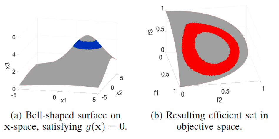
$$ x_1, x_2, x_3 \in [0, 5]. $$ The problem PL-A is constructed with a well-defined structure to allow theoretical analysis of the Pareto-optimal and efficient sets. As shown in the following figure, the function $g(\mathbf{x})$ defines a bell-shaped surface in the decision space ($x$-space). Specifically, the set of solutions satisfying $g(\mathbf{x}) = 0$ forms a ring on the top of this surface (blue region in Fig. a). This set corresponds to the theoretical Pareto set, while the red region in Fig. b shows the efficient set in the objective space. The efficient set is obtained by projecting the feasible solutions onto the objective axes, reflecting the structure imposed by the two priority levels.
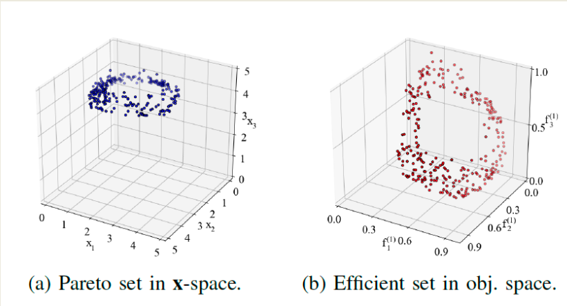
In the following figure, instead, we observe the empirical results obtained by the PL-NSGA-II algorithm when applied to this problem. The plot in Fig. a shows the reconstructed Pareto set in the $x$-space, which is densely and evenly sampled, closely matching the theoretical structure of the previous one (a). Similarly, the plot in Fig. b demonstrates that PL-NSGA-II is able to reconstruct the efficient set in objective space with high fidelity, as it successfully captures the circular structure visible in the previous one (b). These results confirm the effectiveness of the recursive sorting and PL-dominance mechanisms in guiding the algorithm toward high-quality solutions that respect the priority levels.
To quantitatively compare the performance of PL-NSGA-II with other algorithms, we refer to Table I, which reports the results in terms of the Delta metric $\Delta(\cdot) = \max(\text{GD}, \text{IGD})$. The metric combines Generational Distance (GD) and Inverted Generational Distance (IGD) to evaluate both convergence and diversity.
| Algorithm | Mean | Std |
|---|---|---|
| PL-NSGA-II | $0.002 + 0.43①^{-1}$ | $0.002 - 0.09①^{-1}$ |
| MOEA/D-post | $0.01 + 2.18①^{-1}$ | $0.01 + 0.33①^{-1}$ |
| MOEA/D-pre | $0.01 + 2.94①^{-1}$ | $0.01 + 0.90①^{-1}$ |
| NSGA-II-pre | $0.01 + 3.53①^{-1}$ | $0.01 + 0.53①^{-1}$ |
| Lex-NSGA-II | $0.06 + 3.99 \times 10^{4}①^{-1}$ | $0.04 + 74.29①^{-1}$ |
| NSGA-II-post | $0.15 + 2.42 \times 10^{4}①^{-1}$ | $0.03 - 6.94 \times 10^{3}①^{-1}$ |
| NSGA-III-post | $0.49 + 1.47 \times 10^{3}①^{-1}$ | $0.23 + 8.11 \times 10^{3}①^{-1}$ |
| GOAL | $6.63 + 6.62 \times 10^{4}①^{-1}$ | $7.16 - 3.42 \times 10^{4}①^{-1}$ |
| GRAPH | $8.92 + 4.10 \times 10^{4}①^{-1}$ | $6.8 - 7.12 \times 10^{3}①^{-1}$ |
From the results, we can clearly see that PL-NSGA-II significantly outperforms all the competing methods, achieving both the lowest mean and lowest standard deviation. The error terms (expressed in infinitesimal Grossone notation) are also minimal compared to other approaches, indicating both precision and robustness.
These findings confirm that the combination of priority-level-aware sorting, adapted crowding distance, and infinitesimal scalar modeling makes PL-NSGA-II particularly suitable for solving many-objective optimization problems with structured priorities, offering superior convergence and diversity properties.
MaF7
MaF7 is a well-established benchmark in multi- and many-objective optimization, originally designed to test the ability of algorithms to converge and maintain diversity in problems with complex Pareto fronts. In this MPL reformulation, two priority levels are introduced: the first level retains the original three objectives of MaF7, while a second level introduces three additional objectives—thus creating a rich, structured hierarchy of importance.
The objective function to be minimized is:
$$ \min \left[ \begin{pmatrix} x_1 \ x_2 \ h(\mathbf{x}) \end{pmatrix}
- ①^{-1} \begin{pmatrix} f_1^{(2)}(\mathbf{x}) \ f_2^{(2)}(\mathbf{x}) \ h(\mathbf{x}) \end{pmatrix} \right], \quad \text{subject to } \mathbf{x} \in [0,1]^{23} $$
The additional objectives are defined as follows:
- $f_1^{(2)}(\mathbf{x}) = -\exp\left(-0.5 \cdot p(\mathbf{x}, 0.6)\right)$
- $f_2^{(2)}(\mathbf{x}) = \left|p(\mathbf{x}, 0.8) - 0.04\right|$
- $p(\mathbf{x}, c) = (x_1 - c)^2 + (x_2 - c)^2$
- $h(\mathbf{x}) = 6 + \frac{27}{20} \sum_{i=3}^{23} x_i - \sum_{i=1}^{2} x_i (1 + \sin(3\pi x_i))$
The first priority level ($x_1$, $x_2$, and $h$) defines a Pareto front with four disjoint regions, due to the periodic nature of the function $h(\mathbf{x})$. The second priority level introduces functions that isolate one specific region (i.e., the one closest to the line $x_1 = x_2 = 1$), enforcing a stricter selection pressure based on additional structural criteria.
- $f_1^{(2)}$ is a bivariate normal distribution centered at $(0.6, 0.6)$, which favors points close to the center.
- $f_2^{(2)}$ favors points on a circular region centered at $(0.8, 0.8)$ with radius $0.2$.
- The term $h(\mathbf{x})$ promotes solutions farther from the origin, in contrast with $f_1^{(2)}$, which prefers proximity.
These contrasting pressures lead to a nontrivial selection dynamic between priority levels, ideal for testing MPL algorithms.
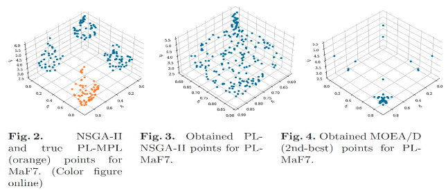
As shown in the following figures, the performance of various algorithms was tested against this MPL version of MaF7. The PL-NSGA-II was able to accurately reproduce the true Pareto-optimal and efficient regions, with a clear clustering of solutions in the intended disjoint zone (see orange and blue points in Fig. 2–3). In contrast, other algorithms such as MOEA/D fail to isolate the preferred region (Fig. 4), demonstrating the superiority of PL-aware mechanisms in guiding the search.
In the following table is presented a comparison across different algorithms using the $\Delta(\cdot) = \max(\text{IGD}, \text{GD})$ metric. This measures the maximum of inverted generational distance and generational distance—indicators of both convergence and spread.
| Algorithm | Mean | Std. Deviation | Avg. # Pareto Solutions |
|---|---|---|---|
| PL-NSGA-II | 1.025e-4 + 3.451e⁻⁵①⁻¹ | 4.201e-5 + 1.788e⁻⁵①⁻¹ | 200.00 |
| GRAPH | 0.332 + 0.558①⁻¹ | 0.038 + 0.079①⁻¹ | 200.00 |
| MOEA/D | 0.003 + 0.001①⁻¹ | 0.001 + 0.001①⁻¹ | 60.00 |
| NSGA-III | 0.357 + 0.543①⁻¹ | 0.021 + 0.034①⁻¹ | 18.32 |
| NSGA-II | 0.010 + 0.005①⁻¹ | 0.004 + 0.002①⁻¹ | 9.44 |
The PL-NSGA-II stands out once again, yielding the lowest error and deviation while covering all 200 expected Pareto solutions. This confirms its capability to balance multiple levels of importance and efficiently guide the search process, in contrast to algorithms not specifically designed to handle priority levels.
These results validate the effectiveness of mixed Pareto-lexicographic optimization strategies and the need for dedicated algorithms like PL-NSGA-II to solve such complex hierarchical problems.
Real-world applications
In addition to synthetic benchmarks, the approach has been applied to real-world problems. One application concerns vehicle crashworthiness, where the goal is to design structures that protect occupants during an impact. In this case, mass and toe-board intrusion resistance were placed at the highest priority level, while acceleration was placed at a lower level. The objective function was modeled as a lexicographic minimization, using the same objective (toe) in two levels, emphasizing its importance. $$ \text{lexmin} \left[ \min \begin{pmatrix} \text{mass}(\mathbf{x}) \ \text{toe}(\mathbf{x}) \end{pmatrix}, \min \begin{pmatrix} \text{toe}(\mathbf{x}) \ -\text{accel}(\mathbf{x}) \end{pmatrix} \right] $$ Another compelling application involves the General Aviation Aircraft (GAA) design problem, which includes 27 constrained input variables and 10 objectives. Based on expert advice, the objectives were grouped into four levels of decreasing importance. The highest-priority objectives included direct operating costs (DOC), lift-to-drag ratio at maximum lift (LDMAX), and range. Objectives such as noise, purchase cost, and weight were placed in the second level, while the least important ones included roughness, fuel weight, and climb speed. A special diversity indicator (PFPF) was placed in the last level and used as a soft constraint to ensure exploration. $$ \text{lexmin} \left[ \min \begin{pmatrix} \textit{PFPF} \end{pmatrix}, \min \begin{pmatrix} \textit{DOC} \ -\textit{LDMAX} \ -\textit{RANGE} \end{pmatrix}, \min \begin{pmatrix} \textit{NOISE} \ \textit{PURCH} \ \textit{WEMP} \end{pmatrix}, \min \begin{pmatrix} \textit{ROUGH} \ \textit{WFUEL} \ -\textit{VCMAX} \end{pmatrix} \right] $$ In both real-world cases, the PL-NSGA-II algorithm showed promising results, effectively handling multiple priority levels and offering practical solutions to complex engineering problems.
Summary and References
The theoretical development of MPL optimization, including both the PC and PL models, has led to new algorithms and applications in diverse domains. A comprehensive review of the state of the art can be found in the paper by Lai, Fiaschi, Cococcioni, and Deb (2022), titled “Pure and Mixed Lexicographic-Paretian Many-Objective Optimization: State of the Art”, published in Natural Computing.
For deeper details on the Priority Chains approach, refer to:
For the Priority Levels model and its real-world validations, see: