Markov Decision Processes and the Foundations of RL

These notes introduce the foundational concepts of Reinforcement Learning (RL), a subfield of machine learning where agents learn to interact with an environment to maximize cumulative rewards. The content is based on the teaching material of Lorenzo Fiaschi for the Symbolic and Evolutionary Artificial Intelligence course at the University of Pisa (a.y. 2024-2025).

At its core, RL models the interaction between an agent and an environment as a loop: the agent selects actions based on observations, the environment responds with new observations and rewards. This loop is typically formalized as a Markov Decision Process (MDP), which will be introduced below.

Mathematical Preliminaries

Markov Process

A fundamental mathematical concept underlying RL is the Markov Process. Consider a state space $S$, which for now is assumed to be discrete. The system undergoes a random walk among these states, meaning that the next state is determined probabilistically.

The key property of a Markov process is the Markovian property, which states that the probability of transitioning to a state $s$ at time $t$ depends only on the state at the previous time step, not on the full history: $$ P(s_t = \bar{s} \mid s_{t-1}, …, s_1) = P(s_t = \bar{s} \mid s_{t-1}) $$ This conditional independence is essential for tractability and is exploited throughout RL algorithms.

The transition kernel is defined as: $$ P(s_t = \bar{s} \mid s_{t-1}) $$ In a concrete example, if $S = {1, 2, 3}$, the system may transition among these three states according to certain probabilities.

Transition Matrix and Stationary Distribution

A Markov process can be fully described by a transition matrix $P \in \mathbb{R}^{|S| \times |S|}$, where each entry $P_{ij}$ represents the probability of transitioning from state $j$ to state $i$. The matrix satisfies: $$ P_{ij} \geq 0, \quad \sum_{i=1}^{|S|} P_{ij} = 1 \quad \forall j \in S $$ An initial starting distribution $s(0)$ over the states is provided. The evolution of the state distribution over time is then given by: $$ s^{(t+1)} = P s^{(t)} = P^t s^{(0)} $$ Under suitable conditions, the process converges to a stationary distribution $s^*$:

$$ s^* = \lim_{t \to \infty} s(t), \quad s^* = P s^* $$

The stationary distribution corresponds to an eigenvector of $P$ associated with eigenvalue $\lambda = 1$. The ergodic theorem ensures the existence and uniqueness of $s^*$ under mild assumptions.

Agent, Environment and the Markovian Hypothesis

In RL, an agent interacts with an environment that is modeled as a Markov Decision Process (MDP), defined by: $$ \text{MDP} = \langle S, A, P, R, \gamma \rangle $$ Where:

• $S$: state space.
• $A$: action space.
• $P$: transition function $P: S \times A \to \mathcal{P}(S)$, where $\mathcal{P}(S)$ is the set of probability distributions over $S$.
• $R$: reward function $R: S \times A \to \mathbb{R}$.
• $\gamma$: discount factor $\gamma \in [0,1]$ that weights future rewards.

The agent is characterized by:

• A policy $\pi$, which may be deterministic $\pi: S \to A$ or stochastic $\pi: S \to \mathcal{P}(A)$.
• A value function $V_\pi: S \to \mathbb{R}$, estimating the expected return starting from state $s$ and following policy $\pi$.
• An action-value function $Q_\pi: S \times A \to \mathbb{R}$, estimating the expected return from taking action $a$ in state $s$ and following policy $\pi$ thereafter.

Analytical Definitions

The mathematical definitions underlying MDPs are as follows:

• Policy: $$ \pi(a \mid s) = P(a_t = a \mid s_t = s) $$
• Expected reward: $$ R(s,a) = R^a_s = \mathbb{E}[r_{t+1} \mid s_t = s, a_t = a] $$
• Expected reward under a policy: $$ R^\pi_s = \sum_{a \in A} \pi(a \mid s) R^a_s = \mathbb{E}_A[R^a_s] $$
• Transition probability: $$ P(s’ \mid s,a) = P^a_{ss’} = P(s_{t+1} = s’ \mid s_t = s, a_t = a) $$
• Expected transition under a policy: $$ P^\pi_{ss’} = \sum_{a \in A} \pi(a \mid s) P^a_{ss’} = \mathbb{E}A[P^a{ss’}] $$
• Value function: $$ V_\pi(s) = \mathbb{E}\pi \left[ \sum{k=0}^\infty \gamma^k r_{t+k+1} ,\bigg|, s_t = s \right] $$
• Return: $$ G_t = \sum_{k=0}^\infty \gamma^k r_{t+k+1} $$
• Action-value function: $$ Q_\pi(s,a) = \mathbb{E}_\pi [G_t \mid s_t = s, a_t = a] $$

Policy Evaluation

Policy evaluation aims to assess how good a given policy $\pi$ is. In particular, the goal is to compute $V_\pi$, which is typically unknown. The basic idea is to let the agent explore the environment following $\pi$, collect the rewards, and use them to infer $V_\pi$.

The value function $V_\pi$ is then used as a measure of the policy’s quality. Under mild assumptions, convergence of the estimated $V_\pi$ is guaranteed.

Bellman Equation

A key tool in RL is the Bellman equation, which provides a recursive relationship for $V_\pi$ and $Q_\pi$. The derivation is based on the following identity: $$ G_t = r_{t+1} + \gamma G_{t+1} $$ Thus, we obtain: $$ V_\pi(s) = \mathbb{E}\pi [ r{t+1} + \gamma V_\pi(s_{t+1}) \mid s_t = s ] $$ Similarly, for the action-value function: $$ Q_\pi(s,a) = \mathbb{E}\pi [ r{t+1} + \gamma Q_\pi(s_{t+1}, a_{t+1}) \mid s_t = s, a_t = a ] $$ Proof: $$ G_t = \sum_{k=0}^\infty \gamma^k r_{t+k+1} = r_{t+1} + \gamma \sum_{k=0}^\infty \gamma^k r_{t+k+2} = r_{t+1} + \gamma G_{t+1} $$ Proving the others is similar.

Bellman Expectation and Closed-form Solution

The Bellman expectation equations rewrite the recursive expressions explicitly: $$ V_\pi(s) = \sum_{a \in A} \pi(a \mid s) \left[ R^a_s + \gamma \sum_{s’ \in S} P^a_{ss’} V_\pi(s’) \right] $$ $$ Q_\pi(s,a) = R^a_s + \gamma \sum_{s’ \in S} P^a_{ss’} \sum_{a’ \in A} \pi(a’ \mid s’) Q_\pi(s’, a’) $$

These equations can also be expressed in matrix form: $$ V_\pi = R^\pi + \gamma P^\pi V_\pi \implies V_\pi = (I - \gamma P^\pi)^{-1} R^\pi $$

Policy Optimization

Ultimately, the goal in RL is to find an optimal policy $\pi^*$ that maximizes the expected return from any starting state.

Having defined the optimal policy $\pi^*$, it is natural to introduce the corresponding optimal value functions, which quantify the best possible expected return achievable from any given state or state-action pair. These functions serve as the theoretical foundation upon which optimal decision-making in RL is built.

It can be shown that for any MDP, there exists an optimal deterministic policy $\pi^*$ such that:

$$ \pi^(a \mid s) = \begin{cases} 1 & \text{if } a = \arg \max_{a \in A} Q^(s,a) \ 0 & \text{otherwise} \end{cases} $$

Bellman Optimality Equations

At optimality, the Bellman equations express the recursive relationships that characterize the optimal value functions. They describe how the value of a state (or state-action pair) under the optimal policy depends on the immediate reward and the optimal values of the subsequent states.

Formally, the Bellman optimality equations are written as: $$ V^(s) = \max_{a \in A} \left[ R^a_s + \gamma \sum_{s’ \in S} P^a_{ss’} V^(s’) \right] $$ $$ Q^(s,a) = R^a_s + \gamma \sum_{s’ \in S} P^a_{ss’} \max_{a’ \in A} Q^(s’,a’) $$ These equations state that:

• The optimal value of a state $s$ is equal to the maximum expected return obtainable by choosing the best possible action $a$ in $s$, receiving the immediate reward $R^a_s$, and then continuing optimally from the next state $s’$.
• Similarly, the optimal action-value function $Q^*(s,a)$ is computed by considering the immediate reward for $(s,a)$ plus the discounted optimal value of the best action at the next state $s’$.

An important property of the Bellman optimality equations is that they are non-linear, due to the presence of the $\max$ operator inside the recursive definitions. As a consequence:

• These equations do not generally admit a closed-form solution.
• In practice, one must rely on iterative approaches to approximate $V^(s)$ or $Q^(s,a)$.

Since these equations cannot be solved analytically in general, many RL algorithms are based on iteratively applying these equations to converge toward the optimal value functions. Classic examples include Value Iteration and Q-Learning, which exploit this recursive structure to improve value estimates over time.

Proof sketch

The derivation of the Bellman optimality equations follows directly from the definitions of the optimal value functions. By definition: $$ V^(s) = \max_{a \in A} Q^(s,a) $$ At the same time, for any action $a$, the optimal action-value function satisfies: $$ Q^(s,a) = R^a_s + \gamma \sum_{s’ \in S} P^a_{ss’} V^(s’) $$ By substituting the expression of $V^(s’)$ (itself defined as the maximum over $Q^(s’,a’)$), and applying this substitution recursively, one obtains the full Bellman optimality equations as stated above.

Policy Optimization Paradigm

A practical method for finding $\pi^*$ is based on the following loop:

1. Start with an arbitrary exploratory policy $\pi$.
2. Evaluate $\pi$ to compute $V_\pi$.
3. Improve the policy by making it greedy with respect to $V_\pi$: $$ \pi \leftarrow \text{greedy}(V_\pi) $$
4. Repeat until $\pi$ converges to $\pi^*$.

Each iteration is known as a Generalized Policy Iteration (GPI) step. Convergence is guaranteed under mild assumptions.

Dynamic Programming (DP)

Dynamic Programming (DP) is a general methodology for solving complex problems by breaking them down into simpler, overlapping subproblems. Unlike the classical “divide and conquer” approach, DP explicitly leverages the fact that subproblems share structure and intermediate results can be stored and reused to avoid redundant computation.

In the context of Markov Decision Processes (MDPs), DP provides a powerful framework for computing optimal value functions and deriving optimal policies. It does so by exploiting the recursive structure of the Bellman equations, which allow the value of each state to be expressed in terms of the values of successor states.

A crucial assumption for the use of DP in this setting is that the agent has full knowledge of the environment — specifically, the transition matrix $P$ and the reward function $R$ must be known in advance.

Policy Evaluation and Improvement with DP

One of the key applications of DP in RL is the iterative evaluation and improvement of a policy. The idea is to alternate between two steps:

1. Policy evaluation: estimate the value function $V_\pi$ for the current policy $\pi$.
2. Policy improvement: update the policy $\pi$ to make it greedy with respect to the current estimate of $V_\pi$.

The policy evaluation step proceeds iteratively. Starting from an initial guess $V_0(s) = 0$ for all $s \in S$, the value function is updated at each iteration according to the Bellman expectation equation: $$ V_{k+1}(s) = \sum_{a \in A} \pi(a \mid s) \left[ R^a_s + \gamma \sum_{s’ \in S} P^a_{ss’} V_k(s’) \right] $$ This process is repeated until convergence, i.e., until the change between successive value functions becomes smaller than a specified threshold $\epsilon$: $$ | V_k - V_{k-1} | \leq \epsilon $$ Once a sufficiently accurate estimate of $V_\pi$ is obtained, the policy improvement step is performed by making the policy greedy with respect to the current value function: $$ \pi(s) \leftarrow \arg \max_{a \in A} \left[ R^a_s + \gamma \sum_{s’ \in S} P^a_{ss’} V_k(s’) \right] $$ This new policy $\pi$ is then used in the next round of evaluation, and the process repeats.

Policy Evaluation at Work: Gridworld

In practical experiments, a simple but highly illustrative example is often used to study policy evaluation and improvement: the Gridworld environment.

What is Gridworld?

Gridworld is a toy environment commonly used in Reinforcement Learning research and teaching. It consists of a finite two-dimensional grid of discrete cells, where each cell corresponds to a distinct state.

The agent can move within the grid by selecting among a set of discrete actions (typically: move up, down, left, right). The environment defines:

• The allowed transitions between cells (some walls or boundaries may block movement).
• Which cells are terminal states that end the episode.
• The reward structure: rewards can be associated with entering particular cells or taking certain actions.

The agent’s goal is to learn a policy that maximizes the cumulative reward, typically by navigating to a target cell while avoiding obstacles or penalties.

Despite its simplicity, Gridworld is a powerful tool for visualizing how value functions evolve during learning, how policies improve through iteration, and how convergence behavior differs between value estimates and policy decisions.

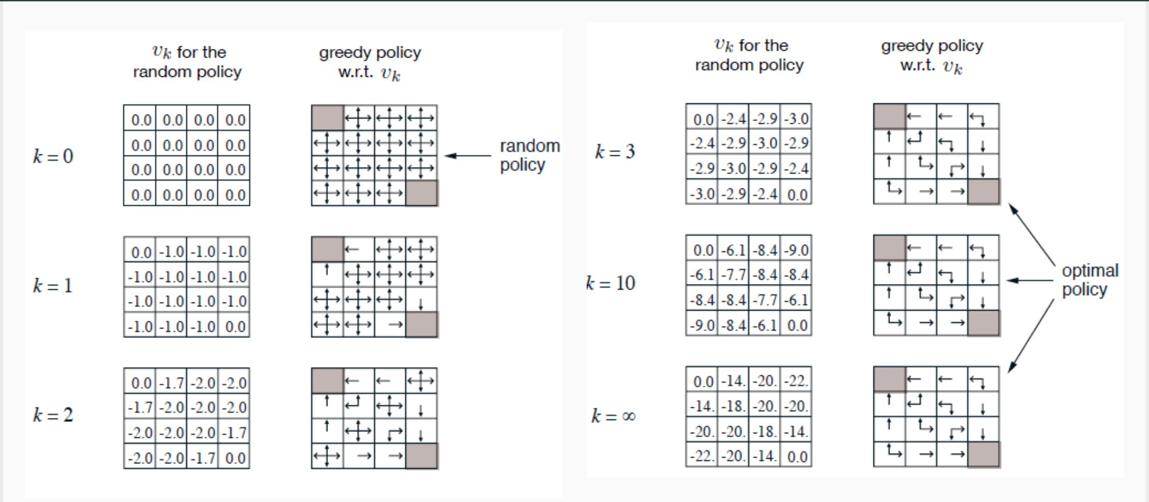
In typical applications of DP to Gridworld, it is often observed that the value function $V_k$ may require many iterations to fully converge. However, the policy often converges much faster — sometimes in just a few iterations — because once the correct policy structure is identified, further refinements of $V_k$ only have marginal impact on the greedy action selection.

Improving the convergence rate of $V_k$ remains an important practical consideration. Techniques such as prioritized sweeping and asynchronous updates can significantly accelerate convergence. It is also important to evaluate whether greedy updates are always the best choice, particularly in contexts where sufficient exploration is still required.

Policy Improvement Guarantee and Value Iteration

A key theoretical result that underpins DP-based policy optimization is the policy improvement theorem. It states that applying the greedy policy improvement step to any non-optimal policy always results in a strictly better policy.

Formally, let $\pi’ := \text{greedy}(V_\pi)$, and suppose that $\pi \ne \pi’$. Then it holds that: $$ V_{\pi’}(s) > V_\pi(s) \quad \text{for all } s \in S $$ Proof

By construction of the greedy policy $\pi’$, we have: $$ Q_\pi(s, \pi’(s)) = \max_{a \in A} Q_\pi(s,a) \geq Q_\pi(s, \pi(s)) = V_\pi(s) $$ If the inequality is strict for at least one state, then clearly $V_{\pi’} > V_\pi$. If instead equality holds for all states, i.e.: $$ V_\pi(s) = \max_{a \in A} Q_\pi(s,a) $$ then this implies that the current policy $\pi$ is already greedy with respect to its own value function — in other words, it is already optimal: $$ V_\pi = V_{\pi’} = V^, \quad \pi = \pi’ = \pi^ $$ Therefore, the policy improvement step either strictly improves the current policy or identifies it as optimal.

Value Iteration

A particularly efficient variant of the DP approach is known as Value Iteration. Rather than performing full policy evaluation and then policy improvement, Value Iteration combines the two steps into a single update rule applied directly to the value function: $$ V_{k+1}(s) = \max_{a \in A} \left[ R^a_s + \gamma \sum_{s’ \in S} P^a_{ss’} V_k(s’) \right] $$ This update is applied iteratively, and the corresponding greedy policy can be extracted at any time from the current estimate of $V_k$. Value Iteration typically converges faster than full policy iteration, particularly when a good initial estimate of the value function is available.

Partial Updates and Limits of DP

While DP provides elegant and powerful algorithms for computing optimal policies, its practical application faces significant challenges, especially in large-scale problems.

Several refinements have been proposed to mitigate the computational cost of DP:

• Asynchronous backups: update the value of each state $V_k(s)$ in-place, rather than waiting for a full sweep over all states.
• Prioritized sweeping: prioritize updates for the states that currently exhibit the largest Bellman residual (i.e., the largest discrepancy between the left-hand side and right-hand side of the Bellman equation).
• Real-time DP: update only the states that are actually visited during interaction with the environment, guided by an exploratory policy $\pi$.
• Early stopping: terminate the iterative process before full convergence if an approximate solution is sufficient for the task at hand.

Despite these refinements, a fundamental limitation remains: DP does not scale well with the size of the state-action space. At each iteration, it typically requires updating every state and considering every possible action, which quickly becomes infeasible in large or continuous environments.

Toward Scalable Solutions

To overcome these limitations, modern RL increasingly relies on more scalable approaches, which relax the assumptions required by DP:

• Sample-based approaches, which estimate value functions or policies using only a subset of observed transitions.
• Model-free methods, which do not require explicit knowledge of the transition matrix $P$ or the reward function $R$.
• Model-based methods, which seek to learn an approximate model of $P$ and $R$ from data, enabling more informed planning and control.

These approaches will be explored in greater detail in the following sections.