Many-Objective Optimization and the NSGA-III algorithm

In engineering, optimization problems often involve multiple conflicting objectives. While classic Multi-Objective Optimization typically refers to problems with 2 or 3 objectives (see Families of Multiobjective Genetic Algorithms), there exist scenarios with a considerably higher number of objectives.

When the number of objectives increases beyond a certain threshold, problems are categorized differently:

• Multi-Objective Optimization: 2 to 3 objectives.
• Many-Objective Optimization: 4 to 30 objectives.
• Massive-Objective Optimization: more than 30 objectives.

These many- and massive-objective problems introduce a set of unique challenges that make them particularly complex to solve.

Intrinsic Difficulties in Many-Objective Optimization

As the number of objectives in an optimization problem increases, several new challenges emerge that are not present—or at least not critical—in standard multi-objective settings. These difficulties are primarily rooted in the properties of high-dimensional objective spaces and have a direct impact on the effectiveness and efficiency of evolutionary algorithms designed to solve such problems.

One of the most significant issues is that, in many-objective spaces, a very large fraction of the population becomes non-dominated. This is problematic because evolutionary multi-objective algorithms (EMOAs) often rely on the concept of Pareto dominance to guide the search process. When most solutions are non-dominated, the algorithm lacks a clear basis for distinguishing and selecting superior individuals. As a result, the selection pressure is drastically reduced, leading to a slower convergence and, ultimately, a less efficient search.

In addition to the dominance-related challenges, maintaining diversity among solutions becomes computationally expensive. Diversity is typically measured using metrics like crowding distance or through the identification of neighboring solutions. However, in high-dimensional spaces, the cost of computing such metrics increases significantly. Any attempt to approximate these computations to save time often results in poor coverage of the Pareto front, yielding a suboptimal and uneven distribution of solutions.

Recombination also becomes inefficient in many-objective settings. Since the objective space is vast, the solutions that are retained in the population are often far apart. When crossover operators are applied to such distant parents, the resulting offspring may also lie far from both parents and from promising regions of the search space. This behavior reduces the effectiveness of traditional recombination techniques, making it necessary to design more sophisticated strategies—such as mating restrictions—to generate useful offspring and maintain convergence.

Another critical difficulty concerns the fact that representing the trade-off surface becomes harder. In a high-dimensional space, accurately approximating the Pareto front requires exponentially more points compared to the bi-objective or tri-objective case. Consequently, a much larger population size is needed, which increases the computational cost and further complicates the task of making decisions based on the results. The abundance of solutions can overwhelm decision-makers, making it difficult to identify a preferred trade-off.

Moreover, performance evaluation becomes more computationally intensive. Metrics like the hypervolume indicator are widely used to compare the quality of different sets of solutions, but their computational cost grows rapidly with the number of objectives. As a result, it becomes more difficult to carry out fair and informative comparisons among algorithms when operating in many-objective scenarios.

Finally, even when the algorithm performs well, visualization becomes impractical. Visualization tools and techniques are generally effective up to three dimensions, sometimes four, but they quickly become inadequate as dimensionality increases. This limits our ability to interpret and understand the trade-offs between objectives, which is a key part of the decision-making process in multi-objective optimization.

In summary, many-objective optimization introduces several interrelated challenges: reduced selection pressure, costly diversity preservation, ineffective recombination, difficult trade-off representation, heavy performance computation, and poor visual interpretability. These issues demand novel algorithmic strategies, such as those introduced in NSGA-III, to ensure effective and practical optimization in high-dimensional objective spaces.

NSGA-III: An Algorithm for Many-Objective Problems

NSGA-III is one of the first algorithms explicitly designed to handle many-objective optimization. It was introduced by Deb and Jain in 2014, and it extends the ideas of NSGA-II with a reference-point-based mechanism for diversity preservation.

Unlike MOEA/D, NSGA-III does not require additional parameters such as neighborhood size or weight vectors. It builds on a set of user-supplied or algorithmically generated reference points on the normalized objective space.

To address the specific challenges of many-objective optimization, NSGA-III extends the classic NSGA-II by introducing a reference-point-based approach for preserving diversity in high-dimensional objective spaces. The algorithm retains the concept of non-dominated sorting but replaces crowding distance with a structured mechanism based on uniformly distributed reference directions. What follows is a detailed explanation of the core steps that NSGA-III performs at each generation, from population evaluation to diversity management and selection.

Step 0: Reference Point Initialization

A set of reference points is generated or supplied. If no user preference is specified, the Das and Dennis method is typically used to place reference points uniformly on a hyperplane of the objective space. These reference points serve to maintain diversity.

Let $M$ be the number of objectives and $p$ the number of divisions per edge of the simplex. The number of reference points $H$ increases combinatorially with $M$ and $p$: $$H=\binom{M+p-1}{p}$$

Step 1: Non-dominated Sorting

The first operational step in each generation of NSGA-III involves identifying the quality structure of the combined population. This is done by merging the parent and offspring populations into a single set $R_t$, which contains all the solutions under consideration.

Once combined, the algorithm performs a non-dominated sorting procedure. This involves partitioning $R_t$ into different non-dominated fronts $F_1,F_2,…$, where each front contains solutions that are non-dominated with respect to each other, but dominated by at least one solution in the previous fronts.

The next population $P_{t+1}$ is then built incrementally. The algorithm adds entire fronts sequentially—starting from the best (i.e., $F_1$)—until the number of individuals in $P_{t+1}$ reaches or slightly exceeds the desired population size $N$. If the last added front causes the population size to exceed $N$, a niching strategy is applied to select only a subset of individuals from that front, ensuring that the final $P_{t+1}$ contains exactly $N$ individuals while preserving diversity.

Step 2: Normalization

In many-objective optimization, direct comparison of objective values can be misleading due to differences in scale. To address this, NSGA-III includes a normalization step that maps all solutions to a common reference frame, improving both the fairness and stability of subsequent association steps.

The normalization procedure begins by computing the ideal point, which consists of the minimum value achieved for each objective among all members of the current population St. This point is then used to translate the objectives, effectively repositioning the origin of the objective space to the ideal point.

Next, the algorithm identifies the extreme points—solutions that lie furthest along each individual objective dimension. These are used to estimate the intercepts, which are scalar values used to rescale each dimension of the objective space.

Finally, each objective value is normalized by dividing it by its respective intercept. This ensures that all objectives are treated uniformly, regardless of their original scale.

Below is the pseudocode corresponding to this normalization process:

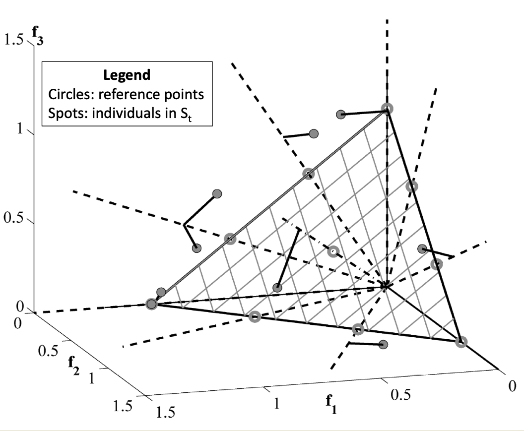
Step 3: Association with Reference Points

Once the population has been normalized, each solution in the current population $S_t$ is associated with the closest reference point in the objective space. This association is based on the perpendicular distance from the solution to the reference direction (i.e., the line defined by a reference point). The result of this step is the construction of a mapping vector $\pi$, which plays a key role in the niching procedure later on.

The vector $\pi$ stores the reference direction assigned to each solution. Specifically, for each solution $s \in S_t$, the vector entry $\pi(s)$ contains the index (or identifier) of the reference point $\mathbf{z} \in Z^s$ to which the solution is closest.

To illustrate this, suppose we have a population $S_t$ of 10 solutions, and from those we have already selected 7 individuals to build the new population $P_{t+1}$. The remaining 3 solutions belong to the last front $F_l$, and they are candidates for filling the final population slots. In this example, the population size is 8, so only one more individual from $F_l$ must be selected.

The association vector $\pi$ in this scenario could look like the following:

$$ \pi = \begin{bmatrix} 2 \ 9 \ 9 \ 3 \ 5 \ 5 \ 2 \ 6 \ 8 \ 9 \ \end{bmatrix} $$

Each entry of $\pi$ indicates the reference direction associated with the corresponding individual in $S_t$. For instance, the first solution in $S_t$ is associated with reference point 2, the second and third with point 9, and so on.

This vector is typically structured such that the first $|P_{t+1}|$ entries correspond to individuals already included in the new population, while the remaining $|F_l|$ entries correspond to the solutions in the last front. In our example:

• The first 7 entries represent the individuals already accepted into $P_{t+1}$
• The last 3 entries represent the candidates in $F_l$

This structure is critical in the next step, where the niching strategy uses $\pi$ to evaluate the distribution of solutions across reference points and decide how to complete the new population in a balanced way.

• $Z^s$: the set of reference points
• $S_t$: the current population

Output:

• $\pi(s \in S_t)$: association of each solution $s$ to a reference point
• $d(s \in S_t)$: perpendicular distance of each solution $s$ to its associated reference line

1. for each reference point $\mathbf{z} \in Z^s$ do

2.     Compute reference line $\mathbf{w} = \mathbf{z}$

3. end for

4. for each $s \in S_t$ do

5.     for each $\mathbf{w} \in Z^s$ do

6.         Compute perpendicular distance:
   $$ d^\perp(s, \mathbf{w}) = \left| s - \frac{\mathbf{w}^T s}{|\mathbf{w}|^2} \mathbf{w} \right| $$

7.     end for

8.     Assign:
   $$ \pi(s) = \arg\min_{\mathbf{w} \in Z^s} d^\perp(s, \mathbf{w}) $$

9.     Assign:
   $$ d(s) = d^\perp(s, \pi(s)) $$

10. end for

Step 4: Niche Count Computation

Using $\pi$, a niche count vector $\rho$ is built. Each element of $\rho$ represents how many individuals are already associated with a given reference direction. This information guides the final selection step.

Step 5: Niching Procedure

After associating each solution in the current population $S_t$ to the closest reference direction, the final step of NSGA-III is to fill the remaining population slots in $P_{t+1}$ using a niching-based selection process. This step is needed when the number of individuals in $P_{t+1}$ has not yet reached the required population size $N$, and we must select a subset of solutions from the last front $F_l$.

To preserve diversity across the objective space, NSGA-III uses the concept of niche count, denoted by $\rho_j$, which keeps track of how many individuals in $P_{t+1}$ are already associated with each reference point $j$ in the set $Z^s$. At each iteration of the niching loop, the algorithm identifies the least crowded reference directions, i.e., those with the smallest $\rho_j$ values.

More precisely, the niching procedure operates as follows:

1. First, the algorithm identifies the set of reference points with the minimum niche count:

   $$ J_{\min} = \left{ j : \rho_j = \min_{j \in Z^s} \rho_j \right} $$

2. One reference point $\bar{j}$ is randomly selected from $J_{\min}$.

3. The algorithm then collects all individuals from the last front $F_l$ that are associated with the reference point $\bar{j}$:

   $$ I_{\bar{j}} = \left{ s \in F_l : \pi(s) = \bar{j} \right} $$

4. If $I_{\bar{j}} \neq \emptyset$, two cases are possible:

   • If $\rho_{\bar{j}} = 0$, meaning no individual in $P_{t+1}$ is yet associated with $\bar{j}$, then the individual $s^*$ in $I_{\bar{j}}$ with the smallest perpendicular distance $d(s)$ from the reference direction is selected:

     $$ s^* = \arg\min_{s \in I_{\bar{j}}} d(s) $$

   • If $\rho_{\bar{j}} \geq 1$, then a randomly chosen individual from $I_{\bar{j}}$ is selected.

5. The selected individual is added to $P_{t+1}$, the niche count $\rho_{\bar{j}}$ is incremented by one, and the solution is removed from $F_l$.

6. If $I_{\bar{j}} = \emptyset$ (i.e., no remaining solution in $F_l$ is associated with $\bar{j}$), then the reference point $\bar{j}$ is excluded from further consideration by removing it from $Z^s$.

7. The process repeats until all $K$ remaining positions in $P_{t+1}$ are filled.

Here is an example of a niche count vector $\rho$ with $|Z^s| = 9$:

$$ \rho = \begin{bmatrix} 0 \ 1 \ 1 \ 0 \ 2 \ 0 \ 0 \ 0 \ 3 \ \end{bmatrix} $$

This tells us, for example, that reference direction 1 is associated with 0 individuals, direction 2 with 1 individual, and so on. The algorithm will prioritize directions like 1 or 4 when adding new individuals.

• $K$ : number of individuals to be selected from $F_l$
• $\rho_j$ : niche count for each reference point
• $\pi(s)$ : reference direction assigned to solution $s$
• $d(s)$ : perpendicular distance of $s$ to its reference direction
• $Z^s$ : set of reference points
• $F_l$ : last front

Output:

$P_{t+1}$

1. $k \gets 1$
2. while $k \leq K$ do
3.     $J_{\min} \gets \left{ j : \rho_j = \min_{j \in Z^s} \rho_j \right}$
4.     Randomly select $\bar{j} \in J_{\min}$
5.     $I_{\bar{j}} \gets \left{ s \in F_l : \pi(s) = \bar{j} \right}$
6.     if $I_{\bar{j}} \neq \emptyset$ then
7.         if $\rho_{\bar{j}} = 0$ then
8.             $s \gets \arg\min_{s \in I_{\bar{j}}} d(s)$
9.         else
10.             Randomly select $s \in I_{\bar{j}}$
11.         end if
12.         $P_{t+1} \gets P_{t+1} \cup {s}$
13.         $F_l \gets F_l \setminus {s}$
14.         $\rho_{\bar{j}} \gets \rho_{\bar{j}} + 1$
15.         $k \gets k + 1$
16.     else
17.         $Z^s \gets Z^s \setminus {\bar{j}}$
18.     end if
19. end while

Main Loop

• $H$ structured reference points $Z^s$

Output:

• $P_{t+1}$

[Step 1] Generate Offspring and Perform Non-dominated Sorting

1. $S_t \gets \emptyset$, $i \gets 1$
2. $Q_t \gets \text{Recombination} + \text{Mutation}(P_t)$
3. $R_t \gets P_t \cup Q_t$
4. $(F_1, F_2, \dots) \gets \text{Non-dominated-sort}(R_t)$
5. repeat
6.     $S_t \gets S_t \cup F_i$
7.     $i \gets i + 1$
8. until $|S_t| \geq N$
9. $F_l \gets F_i$ (last front to be included)
10. if $|S_t| = N$ then
11.     $P_{t+1} \gets S_t$
12.     break

[Step 2] Normalize Objectives

13. $f^n \gets \text{Normalize}(S_t, Z^s)$

[Step 3] Associate Each Member of $S_t$ with a Reference Point

14. $[\pi(s), d(s)] \gets \text{Associate}(S_t, Z^s)$

• $\pi(s)$: closest reference point for each $s \in S_t$
  >- $d(s)$: perpendicular distance between $s$ and $\pi(s)$

[Step 4] Compute Niche Count

15. For each $j \in Z^s$, compute:
    $$\rho_j = \sum_{s \in S_t} (\pi(s) = j ; ? ; 1 ; : ; 0)$$

[Step 5] Apply Niching Procedure to Select $K = N - |P_{t+1}|$ Individuals from $F_l$

16. $P_{t+1} \gets \text{Niching}(K, \rho_j, \pi, d, Z^s, F_l)$

Constraint Handling in NSGA-III

In constrained settings, tournament selection is reintroduced, but the rest of the algorithm remains unchanged. The population size remains equal to the number of directions, and no new parameters are required.

An example application includes the Car Side Impact problem, where feasible regions lie on constraint surfaces, and NSGA-III is able to explore extreme and intermediate trade-offs effectively.

• $p_1$, $p_2$

Ensure:

• $p'$

1. if $feasible(p_1) = \text{TRUE}$ and $feasible(p_2) = \text{FALSE}$ then
2.     $p’ \gets p_1$
3. else if $feasible(p_1) = \text{FALSE}$ and $feasible(p_2) = \text{TRUE}$ then
4.     $p’ \gets p_2$
5. else if $feasible(p_1) = \text{FALSE}$ and $feasible(p_2) = \text{FALSE}$ then
6.     if $CV(p_1) > CV(p_2)$ then
7.         $p’ \gets p_2$
8.     else if $CV(p_1) < CV(p_2)$ then
9.         $p’ \gets p_1$
10.     else
11.         $p’ \gets \text{random}(p_1, p_2)$
12.     end if
13. else if $feasible(p_1) = \text{TRUE}$ and $feasible(p_2) = \text{TRUE}$ then
14.     $p’ \gets \text{random}(p_1, p_2)$
15. end if

Standard crossover (e.g., SBX: Simulated Binary Crossover) and mutation operators are applied, with a high distribution index for SBX to ensure meaningful offspring.