Lexicographic Multi-Objective Optimization and the I-Big-M Method
19 Sep 2025Master AI DataEngineering, Symbolic and Evolutionary Artificial Intelligence9 min read
This section introduces Lexicographic Multi-Objective Optimization Problems (LMOPs), explores standard and non-standard approaches to solving them, and illustrates how Non-Archimedean methods naturally extend classical algorithms. We will gradually connect definitions, algorithms, and examples to form a coherent understanding — culminating with the Infinitely Big-M method.
1. From Single-Objective to Lexicographic Multi-Objective Optimization
Optimization typically focuses on a single scalar function:
$$
\min_{x} f(x) \quad \text{s.t.} \quad x \in D
$$
In many real-world problems, however, multiple objectives must be optimized simultaneously:
$$
f_1, f_2, \dots, f_n
$$
The lexicographic setting imposes a priority order among objectives:
$$
f_1 \gg f_2 \gg \dots \gg f_n
$$
Lexicographic Multi-Objective Optimization Problem (LMOP)
A LMOP is the problem
$$
\operatorname{lex}\min_{x} \ \big(f_1(x), f_2(x), \dots, f_n(x)\big)
$$
subject to $x \in D$, where the priority order is $f_1 \gg f_2 \gg \dots \gg f_n$.
2. A Direct Algorithmic Formulation
The lexicographic definition can be expressed algorithmically by iteratively refining the feasible set:
Algorithm 1: Solving a LMOP
$\Omega \gets D$
For $i = 1, \dots, n$:
If $\Omega = \varnothing$ or $|\Omega| = 1$, break.
Let
$$\Omega_i := \left{\arg\min_{x \in \Omega} f_i(x)\right}$$
Set $\Omega \gets \Omega_i$
Return $\Omega$
This approach directly mirrors the lexicographic order, solving the most important objective first and progressively restricting the feasible set.
3. Preemptive Approach
An equivalent reformulation is to solve each objective sequentially, fixing the optimal value of higher-priority objectives as constraints for the next step.
Preemptive Reformulation
For $i = 1, \dots, n$:
$$\min_{x} f_i(x)$$
subject to
$$f_j(x) = \min_{x \in D} f_j(x), \quad \forall j = 1, \dots, i-1$$
and $x \in D$.
Advantages:
Exactly matches the LMOP definition.
Drawbacks:
Each subproblem becomes more complex.
Problem structure may change.
Inefficient hardware usage (cache misses).
Software inefficiency (no warm start reuse).
4. Weighted Scalarization
Another classical strategy is weighted scalarization: combine all objectives into a single weighted sum, with weights reflecting priority.
Let ${w_i}{i=1}^n$ satisfy $w{i+1} \ll w_i$ for $i = 1, \dots, n-1$.
Weighted Scalarization
Reformulate the LMOP as
$$
\min_{x} \ \sum_{i=1}^n w_i f_i(x) \quad \text{s.t.} \quad x \in D
$$
Drawbacks:
No guarantee that the scalarized problem is equivalent to the original LMOP.
Choosing $w_i$ is arbitrary and error-prone.
Trial-and-error tuning often required.
Very different weight magnitudes can cause numerical instability.
5. Non-Standard Scalarization
A hybrid solution is to exploit Non-Archimedean numbers.
Choose weights:
$$
w_i = \alpha^{,1-i}, \quad i = 1, \dots, n
$$
where $\alpha$ is an infinite number in the Non-Archimedean field.
Non-Standard Scalarization
Reformulate the LMOP as
$$
\min_{x} \ \sum_{i=1}^n f_i(x),\alpha^{,1-i}
$$
subject to $x \in D$.
Advantages:
Equivalent to the original LMOP.
Can be solved with single-objective algorithms.
Retains positive aspects of both preemptive and weighted approaches.
Directly justified by the Transfer Principle.
6. Problems Equivalence Theorem
Consider a LMOP where $f_1, \dots, f_n$ are real-valued and priority is induced by natural order. There exists an equivalent scalar program with
$$
F(x) = \beta_1 f_1(x) + \dots + \beta_n f_n(x)
$$
where $\beta_{i+1} / \beta_i \approx 0$ for $i = 1, \dots, n-1$.
Proof: Let $\Omega$ be the domain, and $\omega \in \Omega$ a global maximum of the LMOP, i.e. $\nexists \omega^\prime \in \Omega$ s.t. $f_1(\omega^\prime)>f_1(\omega)$, or $\nexists i=2, \dots, n$ s.t. $f_j(\omega^\prime) = f_j(\omega)$, with $j = 1, \dots, i-1$ and $f_i(\omega^\prime) > f_i(\omega)$.
However, this is true if and only if $\nexists \omega^\prime \in \Omega$ such that $F(\omega^\prime)>F(\omega)$, by the definition of $F$ itself. This precisely means that $\omega$ is a global maximum for the scalar non-standard program.
7. Lexicographic Multi-Objective Linear Programming (LMOLP)
In the linear case:
$$
\operatorname{lex}\min_{x} \big(c_1^\top x, \dots, c_n^\top x\big) \quad \text{s.t.} \quad Ax = b, \ x \ge 0
$$
can be reformulated as:
$$
\min_{x} \ \sum_{i=1}^n \big(c_i^\top x\big)\alpha^{,1-i} \quad \text{s.t.} \quad Ax = b, \ x \ge 0.
$$
The NA-$c$-Simplex algorithm — a Simplex variant for non-standard cost functions — retains all standard properties, with correctness ensured by the Transfer Principle.
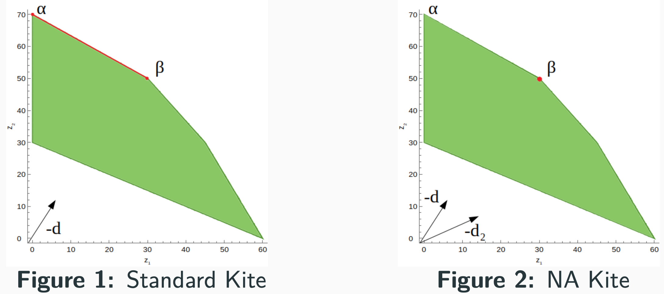
Example: The “Kite” Problem
Standard LMOP form:
$$\operatorname{lex}\max_{x} \big(8x_1 + 12x_2,\ 14x_1 + 10x_2\big)$$
subject to $Ax = b, \ x \ge 0$.
9. The Big-M and Infinitely Big-M (I-Big-M) Methods
In linear programming, situations often arise where the initial basis $B$ required by the Simplex algorithm is not available. A common remedy is to embed the original problem into a larger one by introducing slack variables, ensuring feasibility from the outset.
9.1 Embedding with Slack Variables
Starting from:
$$
Ax = b
$$
we extend the system by adding $m$ slack variables $s \in \mathbb{R}^m$:
$$
Ax + I s = b
$$
where $I$ is the $m \times m$ identity matrix.
This guarantees problem feasibility: the artificial solution $(x,s) = (0,b)$ satisfies the constraints, and the associated starting basis is:
$$
B’ = {n+1, \dots, n+m}
$$
The challenge now is: how to make the enlarged problem equivalent to the original one? Two classical approaches exist:
Two-Phases Method
Big-M Method
9.2 The Two-Phases Method
The Two-Phases method explicitly separates the search for feasibility from the optimization of the original objective.
Phase 1: Feasibility search
$$
\min_{x,s} \ \mathbf{1}^\top s
$$
subject to:
$$
Ax + I s = b, \quad x \ge 0, \ s \ge 0
$$
Any feasible solution to the original problem will have $\mathbf{1}^\top s = 0$.
The starting basis is $B’$ from the slack variables.
If $s = 0$ is achieved, the algorithm proceeds to Phase 2. Otherwise, the original problem is infeasible.
Phase 2: Optimization
Drop the slack variables from the basis:
$$
B := B’[1:n]
$$
Solve the original problem using the Simplex algorithm, starting from $B$.
This method is reliable but computationally more expensive, as it requires running two separate Simplex processes.
9.3 The Classical Big-M Method
The Big-M method attempts to solve the feasibility and optimization in one shot by heavily penalizing the slack variables in the objective:
$$
\min_{x,s} \ , \mathbf{1}^\top s M + d^\top x
$$
subject to:
$$
Ax + I s = b, \quad x \ge 0, \ s \ge 0
$$
where:
$M \ge 0$ is a very large constant (“Big-M”).
$d$ is the cost vector of the original problem.
Big-M Equivalence
There exists $M \ge 0$ sufficiently large such that the solution $\bar{x}^\prime = [0, \bar{x}]$ is solution of the larger problem if and only if $\bar{x}$ is solution of the original problem.
Limitations of the Big-M method:
The choice of $M$ is arbitrary and problem-dependent.
If $M$ is too small → feasibility is not enforced.
If $M$ is too large → numerical instability arises.
Tuning $M$ is essentially a trial-and-error process.
9.4 The Infinitely Big-M (I-Big-M) Method
To understand the role of $M$ in both the Two-Phases and Big-M methods, notice that in both cases the primary goal is to force $s = 0$ before minimizing $d^\top x$. This is precisely a lexicographic priority:
$$
\mathbf{1}^\top s \quad \text{has priority over} \quad d^\top x
$$
The I-Big-M method encodes this directly using a Non-Archimedean infinite number $\alpha$:
$$
\min_{x,s} \ \alpha , \mathbf{1}^\top s + d^\top x
$$
subject to:
$$
Ax + I s = b, \quad x \ge 0, \ s \ge 0
$$
Advantages:
No parameter tuning: $\alpha$ is by definition “big enough”.
No numerical instabilities: infinite scales are handled symbolically.
Guaranteed convergence: $\alpha$ always enforces the lexicographic priority.
Naturally compatible with non-standard optimization frameworks.
I-Big-M at Work: Standard Kite Example
Consider the “Standard Kite” problem. Using I-Big-M, the optimization proceeds as:
| Iteration | $x’$ | $c^\top x’$ | Basis | $x$ |
1
[0, 0, 0, 90, 190, 300, 10, 70, 0]
$-80\alpha$
{4,5,6,7,8}
[0, 0, 0]
2
[0, 35, 0, 55, 85, 195, 10, 0, 0]
$-10\alpha + 420$
{4,5,6,7,2}
[0, 35, 0]
3
[0, 30, 10, 90, 120, 180, 0, 0, 0]
$430$
{4,5,6,3,2}
[0, 30, 10]
4
[0, 70, 10, 50, 0, 60, 0, 0, 0, 80]
$910$
{4,9,6,3,2}
[0, 70, 10]
The final problem form is:
$$\max_{x’} \ - (e + r) \alpha + 8x_1 + 12x_2 + 7x_3$$
subject to:$$
\begin{cases}
2x_1 + x_2 - 3x_3 + s_1 = 90, \
2x_1 + 3x_2 - 2x_3 + s_2 = 190, \
4x_1 + 3x_2 + 3x_3 + s_3 = 300, \
x_3 + e = 10, \
x_1 + 2x_2 + x_3 + r - p = 70, \
x, s, e, r, p \ge 0
\end{cases}$$
Real-World Effectiveness: Benchmark neos-1425699
A real-world benchmark (neos-1425699.mps) is a maximization problem with:
63 inequalities
26 equalities
Known optimal cost: $3.14867 \cdot 10^9$
Using the classical Big-M method, the outcome depends heavily on the choice of $M$:
| $M$ | Optimum Found | Iterations |
$10^2$
$1.36403 \cdot 10^7$
26
$10^3$
$1.29867 \cdot 10^8$
26
$10^4$
$1.25666 \cdot 10^9$
30
$10^5$
$2.95207 \cdot 10^9$
88
$10^6$
$2.95535 \cdot 10^9$
88
$10^7$
$2.98818 \cdot 10^9$
88
$10^8$
$3.14867 \cdot 10^9$
89
$10^9$
$3.14867 \cdot 10^9$
89
With I-Big-M, the optimal solution is found at the first attempt, without any parameter tuning.
10. Conclusions and Future Perspectives
The concepts developed so far — from lexicographic multi-objective optimization to the Non-Archimedean reformulation and the I-Big-M method — find a natural extension in the domain of hierarchical classification, which can be seen as a prioritized decision-making problem. Here, each classification level acts as an “objective” with a strict priority order: correctness at higher levels must take precedence over refinements at lower levels. This interpretation allows the direct reuse of the lexicographic framework to enforce knowledge reuse, maintain coherency across levels, and still pursue high accuracy.
In this setting, Branching Deep Neural Networks (DNNs) provide a structural basis for implementing hierarchical decision processes. Moving from the standard to the non-standard setting introduces a non-standard induced projection operator, enabling the network to internalize infinite-priority constraints between levels. This idea underpins the approach Informed Deep Hierarchical Classification: A Non-Standard Analysis Inspired Approach (Fiaschi and Cococcioni, 2024, under review), which proposes two architectures: Branching CNNs (B-CNNs) and Lexicographic CNNs (L-CNNs).
Experimental results demonstrate that L-CNNs systematically improve coherency without sacrificing accuracy. On a three-level hierarchy, L-CNN achieved 75.07%, 64.00%, and 52.47% accuracy at levels 1, 2, and 3, respectively, with coherency between levels exceeding 87% — significantly higher than B-CNN’s 78–75% range. Moreover, L-CNNs achieve these results with fewer parameters (e.g., 5,746,131 vs. 12,382,035 on CIFAR-100; 2,462,290 vs. 38,755,282 on Fashion-MNIST), highlighting their parameter efficiency.
Ongoing research extends this framework with inference-time abstention mechanisms, allowing the network to decline predictions on never-seen or highly uncertain inputs, in line with the principle that not all mistakes have the same cost. Training is also being adapted for prioritized learning in safety-critical domains such as autonomous driving, where objectives include collision avoidance, maintaining lane centering and street boundaries, adhering to speed limits, and reaching the destination. These directions show how merging non-standard analysis with deep hierarchical models enables decision systems that are not only accurate, but also coherent, informed, and aligned with structured priority constraints.