Function Approximators in Reinforcement Learning

These notes explore the principles and methods of function approximation in Reinforcement Learning (RL), focusing on differentiable approaches for value and policy estimation. The content is based on the teaching material of Lorenzo Fiaschi for the Symbolic and Evolutionary Artificial Intelligence course at the University of Pisa (a.y. 2024–2025).

Function approximators extend the applicability of RL beyond simple, discrete environments. By replacing explicit tables with parameterized functions, RL agents gain the ability to generalize from observed states to unseen ones, enabling learning in large or continuous state spaces.

Limitations of Tabular Methods

Classical tabular methods store value functions in explicit tables, where each entry corresponds to a single state (or state-action pair). While straightforward, this approach presents significant limitations:

• Scalability issues: As the state space grows — potentially to millions or infinitely many states — storing and updating a complete table becomes computationally and memory infeasible.
• Continuous domains: In continuous state spaces, the set of possible states is uncountable, rendering direct tabular storage impossible.
• Lack of generalization: Tabular methods treat every state as unique, with no mechanism to infer similarities. Two nearly identical states must be learned independently, even if they should behave similarly.

To address these limitations, RL relies on function approximation, where the value function $V$ or action-value function $Q$ is represented as a parametric function: $$ V: S \times \Theta \to \mathbb{R}, \quad Q: S \times \Theta \to \mathbb{R}^{|A|} $$ Here, $\Theta$ denotes the parameter space, and $\theta \in \Theta$ is a specific choice of parameters. Function approximation enables the agent to generalize from observed states to new, unseen states.

Types of Function Approximators

A wide range of function approximators can be used in RL. Focusing on differentiable methods, common choices include:

• Kernel and feature maps
• Deep Neural Networks (DNNs)
• Decision Trees
• k-Nearest Neighbours (k-NNs)
• Fourier and wavelet transforms

While these approaches are powerful, they face two notable challenges in RL:

1. Non-stationary data
   Policies evolve during training, altering the distribution of visited states. In some cases, the environment itself may change over time, further shifting the data distribution.

2. Non-IID (independent and identically distributed) samples
   Unlike supervised learning, where samples are often assumed IID, RL generates sequential, correlated data. This violates standard statistical assumptions and can destabilize learning.

Incremental Learning with Stochastic Gradient Descent

Consider the task of policy evaluation: estimating $V_\pi$ for a given policy $\pi$. A natural approach is to minimize the mean squared error (MSE) between the estimated and true value functions: $$ L(\theta) = \mathbb{E}\big[(V_\pi(s) - V(s,\theta))^2\big] $$ In linear value approximation, the value function is modeled as: $$ V(s,\theta) = \phi(s)^\top \theta $$ where $\phi(s)$ is a feature vector encoding the state $s$. Thanks to the Representer Theorem, linear approximation is often sufficient in feature space. In this case, $L(\theta)$ is quadratic, and its gradient is: $$ \Delta\theta = \nu , (V_\pi(s) - V(s,\theta)) , \phi(s) $$ where $\nu$ is the learning rate.

In practice, $V_\pi$ is not available and must be replaced with an empirical target $G_t$.

• Monte Carlo (MC) evaluation

  • $G_t$ is an unbiased estimate but noisy.
  • The method performs supervised learning on $(s_t, G_t)$.
  • Strong convergence guarantees.

• TD(0) evaluation

  • $G_t$ is replaced by $r_{t+1} + \gamma V(s_{t+1},\theta)$.
  • Biased but less noisy.
  • Weaker convergence guarantees.

• TD($\lambda$)

  • Uses $\lambda$-returns $G_t^\lambda$, blending MC and TD targets.
  • Eligibility traces are adapted to the state encoding:$$ E_t = \gamma\lambda E_{t-1} + x(s_t) $$

Batched Learning and Experience Replay

To stabilize gradient estimates, batched learning collects multiple samples before computing an update. This reduces variance and helps address the non-stationarity and non-IID problems.

A common solution is the experience replay buffer:

• Stores past transitions $(s,a,r,s’)$ in a dataset.
• Allows random sampling, breaking temporal correlations.
• Enables repeated use of past experiences.
• Supports prioritized sampling, giving more importance to high-error transitions.

Experience replay, combined with state space encoding, greatly improves training stability in neural-network-based RL.

Deep Q-Networks (DQN)

A Deep Q-Network (DQN) uses a neural network to approximate the action–value function $Q(s,a;\theta)$. DQN is an off-policy TD method that stabilizes learning with three core ideas:

• Experience replay buffer: store past transitions $(s,a,r,s’)$ and train on mini-batches sampled from this buffer to break temporal correlations and reduce variance. Both uniform and prioritized sampling are possible.
• Fixed Q-targets: maintain a target network with parameters $\theta^-$, a copy of the online network’s parameters $\theta$ that is held fixed for several updates. Targets “come from an old, fixed version of the network” and $\theta^-$ is periodically updated (every $C$ steps) or via soft updates.
• $\varepsilon$-greedy exploration: act mostly greedily w.r.t. $Q(\cdot;\theta)$ while ensuring continued exploration with probability $\varepsilon$.

Simple DQN target and loss

Using a replay buffer $\mathcal{D}$, the simple DQN target for a sampled transition $(s,a,r,s’)$ is $$ y^{\text{DQN}} ;=; r ;+; \gamma ,\max_{a’\in A} Q(s’,a’;\theta^-),, $$ and the loss is $$ L(\theta) ;=; \mathbb{E}_{(s,a,r,s’)\sim \mathcal{D}}\Big[\big(y^{\text{DQN}} - Q(s,a;\theta)\big)^2\Big]. $$

Effect of maximization bias (intuitive example)

• Let A be the starting state.
• Suppose a lucky, positive outcome is observed when going left from A.
• Because the learning target uses a max over action values, the overestimated action inflates its own target and can spill into nearby states, biasing learning toward B (the region reached by “left”), even if the true advantage is smaller.

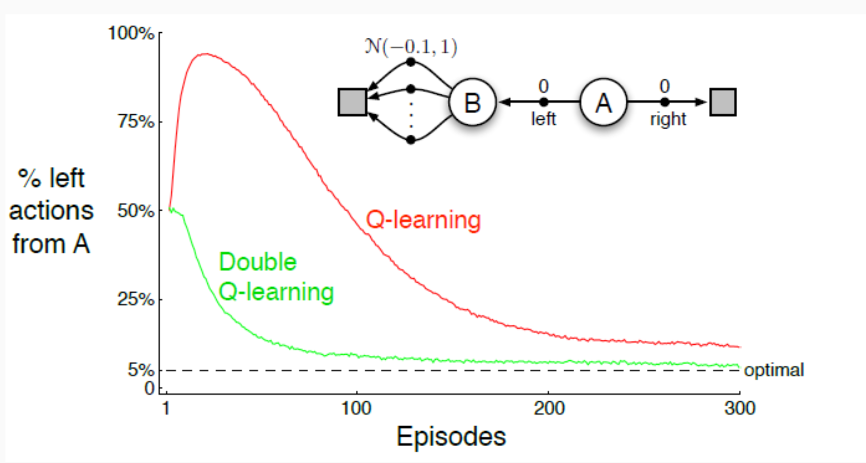
Double DQN decouples action selection (online network) from action evaluation (target network): $$ y^{\text{DDQN}} ;=; r ;+; \gamma , Q!\Big(s’,;\arg\max_{a’\in A} Q(s’,a’;\theta);,;\theta^- \Big), $$ with loss $$ L(\theta) ;=; \mathbb{E}_{\mathcal{D}}\Big[\big(y^{\text{DDQN}} - Q(s,a;\theta)\big)^2\Big]. $$ This simple change avoids using the same noisy estimates for both choosing and evaluating the greedy action, which reduces the maximization bias and typically yields more reliable value estimates.

Dueling networks: value + advantage

The dueling architecture re-parameterizes $Q$ as a state value plus a per-action advantage: $$ Q(s,a;\theta) ;=; V(s;\theta_V);+;A(s,a;\theta_A);-;\max_{a’\in A} A(s,a’;\theta_A). $$

• $V(s;\theta_V)$ captures how good a state is regardless of action.
• $A(s,a;\theta_A)$ captures the relative value of selecting action $a$ in $s$.
• Subtracting $\max_{a’} A(s,a’)$ ensures identifiability (prevents arbitrary shifts between $V$ and $A$) and matches the slide’s formulation.

Practical training loop (concise)

1. Collect transitions $(s,a,r,s’)$ with $\varepsilon$-greedy policy from $Q(\cdot;\theta)$ and push to replay buffer $\mathcal{D}$.
2. Sample a mini-batch from $\mathcal{D}$.
3. Compute targets: $y^{\text{DQN}}$ or $y^{\text{DDQN}}$ (using $\theta^-$).
4. Update $\theta$ by minimizing $L(\theta)$ (often with Adam; Huber loss is also common in practice).
5. Periodically update $\theta^- \leftarrow \theta$ (or soft-update).

Policy Gradient Methods

In policy gradient methods, the optimal policy $\pi^$ is approximated directly, rather than being derived from an optimal value function $V^$ or action–value function $Q^$. The policy is expressed as a parameterized function $\pi(a \mid s; \theta)$, where the parameters $\theta$ are adjusted to maximize the expected return. This direct approach often converges faster than first estimating $V^$ and deriving a greedy policy, and is particularly effective in complex or continuous action spaces, as well as in settings where stochastic policies are advantageous, such as in multi-agent or game-theoretic contexts.

The main benefits of this approach lie in its potential for faster convergence and its applicability to large or continuous action spaces, together with its natural support for stochastic policies. However, these advantages are tempered by certain drawbacks. There is no guarantee of reaching a globally optimal policy, the variance in gradient estimates can be high, and the method requires the policy to be differentiable with respect to its parameters. Furthermore, policy evaluation may become computationally inefficient without additional stabilizing mechanisms.

A central question is how to evaluate and improve a policy in the absence of explicit knowledge of $V_\pi$ or $Q_\pi$. One approach is based on Monte Carlo estimation. In the deterministic case, the objective can be written as $L(\theta) = \mathbb{E}\pi[V(s_1)]$, while in the stochastic case it becomes $L(\theta) = \mathbb{E}\pi[ V(s_1) \mid s_1 \sim \mathcal{P}(S)]$. This amounts to estimating the average value or reward associated with the initial state distribution. An alternative is to rely on Temporal Difference estimation, where the objective is defined as the sum over all states of the stationary distribution $d_\pi(s)$ weighted by either the value function $V(s)$ or the expected reward $\sum_{a \in A} \pi(a|s,\theta) R_s^a$.

The Policy Gradient Theorem formalizes the update direction for $\theta$. If $\pi$ is differentiable, then $$ \nabla_\theta L(\theta) \propto \sum_{s \in S} d_\pi(s) \sum_{a \in A} \nabla_\theta \pi(a|s,\theta) , Q_\pi(s,a). $$ Considering that: $$\sum_{s \in S} d_\pi(s) \sum_{a \in A} \nabla_\theta \pi(a|s,\theta) , Q_\pi(s,a) = \mathbb{E}{\pi}\left[ \sum{a \in A} \nabla_\theta \pi(a|S,\theta) , Q_\pi(S,a) | d_{\pi}(S) \right]$$Applying the log-derivative trick, $\nabla_\theta \pi(a|s,\theta) = \pi(a|s,\theta) \nabla_\theta \ln \pi(a|s,\theta)$, leads to the compact expression $$ \nabla_\theta L(\theta) \propto \mathbb{E}{\pi}\big[ \nabla\theta \ln \pi(a|s,\theta) , Q_\pi(s,a) | d_{\pi}(S,A) \big], $$ which forms the foundation for most policy gradient algorithms.

In the Monte Carlo policy gradient variant, $Q_\pi(s_t,a_t)$ is replaced by the empirical return $G_t$, which is an unbiased sample of the action–value function. The resulting update rule is $$ \nabla_\theta L(\theta) \approx \frac{1}{N} \sum_{i=1}^N \sum_{t=1}^T \nabla_\theta \ln \pi(s_t^{(i)}, a_t^{(i)}; \theta) , G_t^{(i)}. $$ Since this formulation relies on on-policy data, the trajectories used to compute $G_t$ are drawn from the current policy $\pi$. The effect of $G_t$ in the update is to give more weight to actions taken in episodes that yield higher returns, which can also be interpreted as a form of maximum likelihood estimation over successful trajectories. In the off-policy setting, importance sampling must be introduced to correct for the mismatch between the behavior policy $\mu$ and the target policy $\pi$, although this typically introduces substantial variance, especially for long-horizon problems, and is seldom used without additional variance-reduction techniques.

Actor–Critic Methods

Actor–Critic methods integrate policy gradient techniques with value function approximation. The central idea is to maintain two distinct components. The Actor is responsible for updating the policy parameters $\theta$ so as to maximize the expected return, while the Critic evaluates the quality of the actions taken under the current policy, typically by estimating either $Q_\pi(s,a)$ or $V_\pi(s)$. This arrangement allows the Actor to benefit from the Critic’s feedback, thereby reducing the variance of pure Monte Carlo policy gradient estimates.

When the action–value function is approximated as $Q(s,a,\omega)$, the implementation can follow two main architectures. If $\omega \neq \theta$, the Actor and Critic use separate neural networks, which is conceptually simple, stable, and avoids feature-sharing conflicts. If $\omega = \theta$, a single network is used to parameterize both components, enabling feature sharing but potentially causing gradient interference between the Actor and Critic objectives.

Compatible Function Approximation

The Compatible Function Approximation Theorem states that, in the Actor–Critic framework, if two conditions hold:

1. Compatibility: $$\nabla_\omega Q(s,a,\omega) = \nabla_\theta \ln \pi(a|s,\theta)$$
2. Unbiasedness: $$\mathbb{E}\pi\big[(Q\pi(s,a) - Q(s,a,\omega))^2\big] \xrightarrow[t \to \infty]{} 0$$then the Policy Gradient Theorem remains valid, and the gradient can be expressed as$$\nabla_\theta L(\theta) \propto \mathbb{E}\pi\big[\nabla\theta \ln \pi(A|S,\theta) , Q(S,A,\omega) \mid d_\pi(S,A)\big].$$ Under these conditions, the action–value function can be written as $$ Q(s,a,\omega) = \nabla_\theta \ln \pi(a|s,\theta)^\top \omega. $$

Baselines and Variance Reduction

The variance of the policy gradient can be further reduced by introducing a baseline function $B(\cdot)$, which represents empirical knowledge about the expected returns and is subtracted from the action–value estimates without introducing bias.

The modified gradient takes the form $$ \nabla_\theta L(\theta) \propto \mathbb{E}\pi\left[ \sum{a \in A} \nabla_\theta \pi(a|S,\theta) , \big(Q_\pi(S,a) - B(\cdot)\big) ; \middle| ; d_\pi(S) \right]. $$

If the baseline depends only on the state, i.e. $B = B(S)$, it does not alter the gradient, because $$ \mathbb{E}\pi\left[ \sum{a \in A} \nabla_\theta \pi(a|S,\theta) B(S) \right] = \mathbb{E}\pi\big[ B(S) \nabla\theta 1 \big] = 0. $$

A natural and effective choice for the baseline is the state-value function itself: $$ B(s) = V_\pi(s). $$

Advantage Function

With the baseline $B(s) = V_\pi(s)$, the advantage function emerges naturally: $$ A_\pi(s,a) = Q_\pi(s,a) - V_\pi(s), $$ which measures the added value of taking action $a$ in state $s$ relative to the baseline value $V_\pi(s)$.

The gradient of the objective then becomes $$ \nabla_\theta L(\theta) \propto \mathbb{E}\pi \left[ \nabla\theta \ln \pi(A|S,\theta) , A_\pi(S,A)\middle| ; d_\pi(S, A) \right]. $$

Advantage Policy Gradient in the Actor–Critic Scenario

In a practical Actor–Critic algorithm, the advantage function is often parameterized explicitly. This requires, in general, three parameter sets: $$ A(s,a,\omega,\rho) = Q(s,a,\omega) - V(s,\rho), $$ although in many cases only the parameters $\rho$ for $V(s,\rho)$ are needed.

The action–value and advantage functions can be expressed as $$ Q_\pi(s,a) = \mathbb{E}{s’ \in S} \big[ r + \gamma V\pi(s’) ; \big| ; s,a \big], $$ $$ A_\pi(s,a) = \mathbb{E}{s’ \in S} \big[ r + \gamma V\pi(s’) - V_\pi(s) ; \big| ; s,a \big]. $$ The degree of bootstrapping in these estimates depends on the time-scale chosen for updating the value function and policy parameters. A shorter time-scale for the Critic leads to more immediate but potentially noisier updates, while a longer time-scale smooths learning but can slow down policy improvement.

Natural Policy Gradient

Standard policy gradient methods, while conceptually straightforward, often struggle with slow convergence and instability. This is particularly evident when the policy induces noisy data, or when the optimization process encounters plateaus and discontinuities in policy space. In such cases, the vanilla policy gradient treats all parameter directions as equally important, ignoring the geometry of the space of policies. This can result in inefficient updates that change some aspects of the policy too much while barely affecting others, leading to high non-stationarity.

The Natural Policy Gradient (NPG) approach addresses this issue by making changes to the parameters $\theta$ proportional to changes in the policy itself, rather than to changes in parameter space alone. The similarity between the old and new policies is quantified using the Kullback–Leibler (KL) divergence: $$ \mathrm{KL}(\pi(\theta_t) ,|, \pi(\theta_{t+1})) = \int_{S \times A}\pi(a|s,\theta_t) , \ln \left(\frac{\pi(a|s,\theta_t)}{\pi(a|s,\theta_{t+1})} \right), d(s,a), $$ which measures the loss of information when moving from $\pi(\theta_t)$ to $\pi(\theta_{t+1})$. The natural gradient seeks the optimal update direction that maximizes the performance objective while constraining the change in policy to satisfy: $$ \mathrm{KL}(\pi(\theta_t) ,|, \pi(\theta_{t+1})) \leq \varepsilon. $$

Geometric Interpretation

In the parameter space, the set of directions that satisfy the KL constraint forms an ellipse of feasible gradients. The vanilla gradient method ignores this curvature, moving in straight lines that may be inefficient with respect to the policy’s actual behavior. The NPG method re-scales and re-orients the gradient according to the local geometry, thereby avoiding plateaus and making more meaningful improvements.

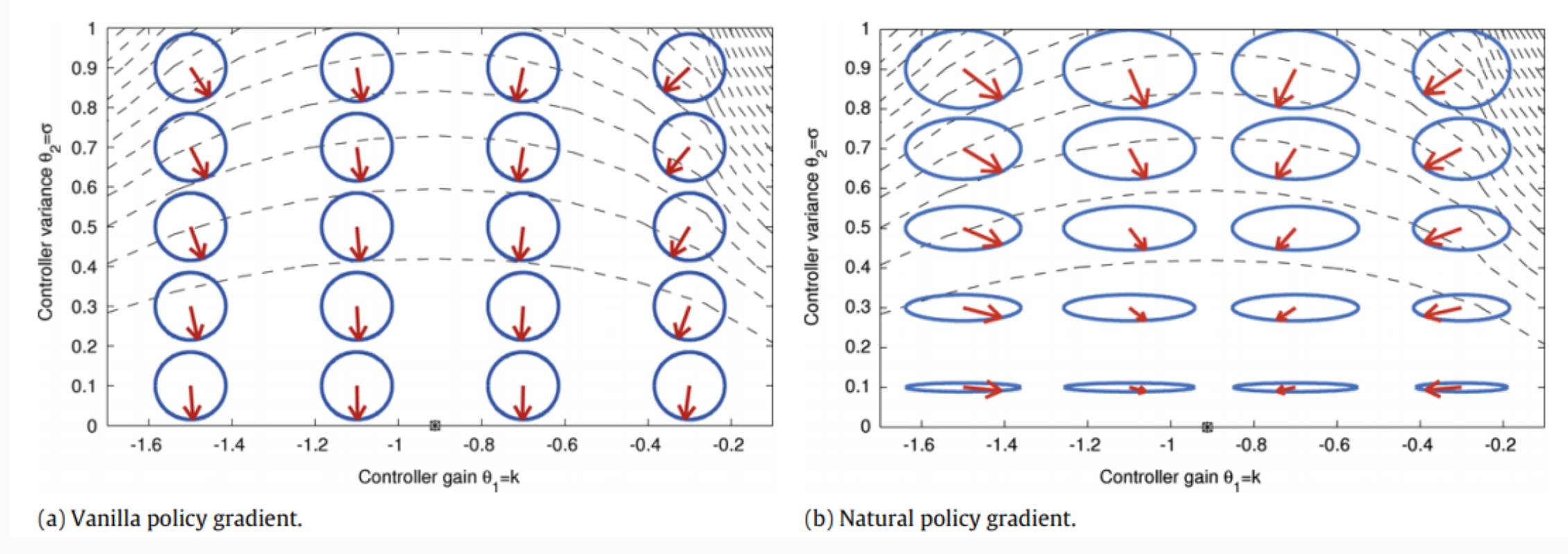
The NPG update rule can be derived by solving a constrained optimization problem in which the objective $\nabla_\theta L(\theta)$ is maximized subject to the KL bound. The solution is: $$ \Delta\theta \propto G_\theta^{-1} , \nabla_\theta L(\theta), $$ where $G_\theta$ is the Fisher information matrix: $$ G_\theta = \mathbb{E}\pi \left[ \left< \nabla\theta \ln \pi(a|s,\theta) ,, \nabla_\theta \ln \pi(a|s,\theta)^\top \right> \right]. $$

From the Policy Gradient Theorem, the natural gradient update can be written as: $$ \Delta\theta \propto G_\theta^{-1} , \mathbb{E}\pi\left[ \nabla\theta \ln \pi(a|s,\theta) , Q_\pi(s,a) \right]. $$

Under the compatible function approximation condition for the critic, $$ Q(s,a,\omega) = \nabla_\theta \ln \pi(a|s,\theta)^\top \omega, $$ the update simplifies further: $$ \Delta\theta \propto G_\theta^{-1} , \nabla_\theta \ln \pi , \nabla_\theta \ln \pi^\top \omega = G_\theta^{-1} G_\theta \omega = \omega. $$ This shows that, under compatibility, the natural gradient reduces to updating $\theta$ in the direction of the critic’s weight vector $\omega$.