From Data to Models - Foundations of Function Approximation and Classification

The first part of this course focuses on creating a model to describe the relationship between an input pattern $p$ and its associated output $o$. This concept is fundamental for machine learning, where we aim to predict outcomes or derive insights based on input data. The process of modeling involves understanding the structure of the data and creating functions that can approximate or fit the data effectively.

Why Modelling Instead of Lookup Tables?

A common question arises: if we have a dataset composed of pairs $(P_n, o_n)$, why build a model instead of storing these pairs in a Look-Up Table (LUT) and using methods like 1-NN (Nearest Neighbor)? The main reason is that a LUT cannot interpolate or denoise the samples. While using $k$-NN helps to mitigate this by introducing interpolation between the outputs of the $k$ nearest neighbors, relying on a LUT combined with $k$-NN offloads all complexity to the inference phase. Additionally, being model-free, a LUT cannot compress, simplify, or exploit regularities present in the learning set, resulting in inefficiencies and potentially poor performance for unseen data.

Splitting the Learning Set

Given a learning set ${P_n, Y_n}$, we typically split it into two parts:

• Training Set (TRS): ${P_n, Y_n}{n=1}^{N{tr}}$
• Test Set (TSS): ${P_n, Y_n}{n=1}^{N{ts}}$

Here, $P_n \in \mathbb{R}^D$ represents the patterns or observations, and $Y_n$ is either the output for regression problems or the label for classification problems. The union of TRS and TSS gives the entire learning set, while their intersection is empty ($N_{tr} + N_{ts} = N$). Sometimes, a third dataset called the Validation Set (VLS) is also used to evaluate the model during training, allowing further tuning of hyperparameters and preventing overfitting. In regression problems, $Y_n$ is referred to as the output associated with the $n$-th input pattern. For classification problems, $Y_n$ is the label associated with that input pattern. To efficiently work with these datasets, we often organize all patterns of the training set into a single matrix $P$, and all outputs into a column vector $\mathbf{o}$:

$$P = \begin{bmatrix} p_1^1 & \dots & p_1^d & \dots & p_1^D

\ p_2^1 & \dots & p_2^d & \dots & p_2^D

\ \cdots & \cdots & \cdots & \cdots & \cdots

\ p_N^1 & \dots & p_N^d & \dots & p_N^D

\end{bmatrix} \in \mathbb{R}^{N \times D}, \quad \mathbf{o} = \begin{bmatrix} o_1 \ o_2 \ \vdots \ o_N \end{bmatrix} \in \mathbb{R}^N$$ In most regression problems, we typically have more patterns than dimensions ($N \gg D$), making matrix $P$ "tall", which is helpful for finding generalizable solutions.

Interpolation vs Approximation

Interpolation is a technique used to estimate the value of a function at any point within a set of known data points. The goal is to construct a function that passes exactly through these data points. The assumption in interpolation is that the function being modeled is continuous within the given interval, meaning there are no sudden jumps or missing values between the known points. Common interpolation techniques include polynomial and spline interpolation.

Approximation, on the other hand, is used to find a simpler representation of a dataset or function that captures its overall behavior rather than fitting it exactly. The goal is to derive an approximate model that may not pass through every data point but still provides an understanding of the general trend. Approximation methods, such as least squares regression or Fourier series, focus on minimizing the error between the real data and the predicted values.

The choice between interpolation and approximation depends on the problem at hand. If the goal is to fit data exactly, interpolation is preferable. However, if we are interested in understanding trends or building a robust predictive model, approximation techniques are generally more suitable.

Linear Least Squares Approximation

One of the simplest ways to approximate a function known by a discrete set of input-output pairs $(p, o)$ is to use a linear function: $$f(p) = b + \mathbf{v}^T p$$ Here, $b$ is the bias term and $\mathbf{v}$ is a vector of weights. The parameters $b$ and $\mathbf{v}$ can be estimated in such a way that minimizes the Mean Squared Error (MSE) between the true output and the approximated output: $$E = \frac{1}{2} (o - f(p))^2$$ This process is known as Linear Least Squares Fitting.

The closed-form solution for $b$ and $\mathbf{v}$ can be found using the pseudo-inverse technique, which provides an optimal, non-iterative solution. Specifically, the vector with both the bias and the weights $w = [b, \mathbf{v}]$ can be calculated as: $$\mathbf{w} = \mathbf{y} \mathbf{X}^T (\mathbf{X} \mathbf{X}^T)^{-1}$$ where $\mathbf{X}$ is the matrix of input patterns and $\mathbf{y}$ is the vector of outputs. $$\mathbf{X} = \begin{bmatrix} 1 & 1 & \cdots & 1 \ p_1^1 & p_2^1 & \cdots & p_N^1 \ \vdots & \vdots & \ddots & \vdots \ p_1^D & p_2^D & \cdots & p_N^D \end{bmatrix}, \quad \mathbf{y} = o^T = \begin{bmatrix} o_1 & o_2 & \cdots & o_N \end{bmatrix}$$ This formula is both mathematically elegant and computationally efficient for small to medium-sized datasets.

However, the computational complexity of this closed-form solution is $O(N^2(D + 1))$, which can be prohibitive for very large datasets. This is why iterative methods like Gradient Descent are often preferred in practice.

Weighted Linear Least Squares

In some scenarios, it is useful to assign different levels of importance to different data points. This can be achieved using Weighted Linear Least Squares, where each input-output pair is assigned a weight $\delta_n$. The objective is then to minimize a weighted version of the MSE: $$E = \frac{1}{2} \sum_{n=1}^{N} \delta_n (o_n - f(p_n))^2$$ The closed-form solution can be adjusted to account for these weights by incorporating a diagonal matrix $\Delta = \text{diag}(\delta_1, \delta_2, \ldots, \delta_N)$, leading to: $$\mathbf{w} = (\mathbf{X}^T \Delta \mathbf{X})^{-1} \mathbf{X}^T \Delta \mathbf{y}$$ This formulation allows us to handle datasets where certain observations are more reliable or more important than others.

Advantages of the Closed-Form Solution

The closed-form solution for Linear Least Squares has several advantages:

• Mathematically Elegant: It provides a direct solution without requiring iterative optimization, which is both elegant and efficient for small problems.
• Psychologically Reassuring: Knowing that an exact, optimal solution exists can be comforting, especially when dealing with simpler models.
• Non-Iterative: Unlike Gradient Descent, there is no need to choose a learning rate or worry about convergence.
• Optimal Solution: The solution obtained is exact and not an approximation, unlike iterative methods which may only approximate the optimal values.
• Utilizes Matrix Operations: Efficient linear algebra routines are available, which makes computation faster and more reliable.

Linear Least Squares with Gradient Descent

Despite the availability of a closed-form solution, Gradient Descent is often used for large-scale problems where computing the pseudo-inverse is impractical. The Gradient Descent method works by iteratively updating the weights in the direction of the steepest descent of the error function. The error for the $n$-th data point is given by: $$E_n = \frac{1}{2} ((b + \mathbf{v} p_n^T) - y_n)^2$$ The update rules for the parameters $b$ and $\mathbf{v}$ are: $$\begin{aligned}

b &\leftarrow b - \eta \frac{\partial E_n}{\partial b} \

\mathbf{v} &\leftarrow \mathbf{v} - \eta \frac{\partial E_n}{\partial \mathbf{v}}

\end{aligned}$$ where $\eta$ is the learning rate. The choice of $\eta$ is crucial: if it is too small, convergence will be very slow; if too large, the solution may oscillate or even diverge.

The derivatives of the error with respect to $b$ and $\mathbf{v}$ are: $$\frac{\partial E_n}{\partial b} = ((b + \mathbf{v} p_n^T) - y_n), \quad \frac{\partial E_n}{\partial \mathbf{v}} = ((b + \mathbf{v} p_n^T) - y_n) p_n^T$$

Computational Complexity

The computational complexity of Gradient Descent for each iteration is $O(N(D + 1))$ ($O(D+1)$ for each sample times $N$ elements of the dataset), and for $k$ iterations, it is $O(kN(D + 1))$. This is typically much lower than the complexity of the closed-form solution, especially for large $N$, making Gradient Descent a more scalable option for big datasets.

Gradient Descent for Linear Least Squares

Although Linear Least Squares has a closed-form solution, Gradient Descent can also be used to estimate $b$ and $\mathbf{v}$ iteratively. The steps are:

1. Initialize weights $b$ and $\mathbf{v}$ to random values.
2. Set a learning rate $\eta$, which controls the step size during the update.
3. Compute the predicted values for each data point using the current parameters: $$\hat{y}_n = b + \mathbf{v} p_n^T$$4. Update the parameters $b$ and $\mathbf{v}$ using the computed gradients and the learning rate. $$\begin{aligned}

b &\leftarrow b - \eta \frac{\partial E_n}{\partial b} \

\mathbf{v} &\leftarrow \mathbf{v} - \eta \frac{\partial E_n}{\partial \mathbf{v}}

\end{aligned}$$5. Repeat until convergence or for a fixed number of iterations.

The learning rate plays a crucial role: if it is too small, convergence will be slow; if too large, the algorithm may diverge. Once the algorithm has converged, the final weights $b$ and $\mathbf{v}$ can be used to appoximate the given function using the linear function $f(p) = b + \mathbf{v}^T p$.

Pseudocode

$$ \begin{aligned} \textbf{Pseudocode: Linear Regression with Gradient Descent} \ \textbf{Input:} & \quad {(p_n, y_n)}_{n=1}^N, \eta, \text{num_iters} \ \textbf{Output:} & \quad b, \mathbf{v}, \text{avg_error_history} \ \ b \leftarrow 0 \ \mathbf{v} \leftarrow \text{zeros}(D) \ \text{avg_error_history} \leftarrow \text{zeros}(\text{num_iters}) \ \ \textbf{for } k = 1 \text{ to } \text{num_iters:} \ \quad \text{sum_error} \leftarrow 0 \ \quad \textbf{for each } n = 1 \text{ to } N: \ \quad\quad \hat{y} \leftarrow b + \mathbf{v} \cdot P[n,:]^T \ \quad\quad E \leftarrow 0.5 \cdot (\hat{y} - y[n])^2 \ \quad\quad \text{sum_error} \leftarrow \text{sum_error} + E \ \quad\quad \text{gradient_b} \leftarrow \hat{y} - y[n] \ \quad\quad \text{gradient_v} \leftarrow (\hat{y} - y[n]) \cdot P[n,:] \ \quad\quad b \leftarrow b - \eta \cdot \text{gradient_b} \ \quad\quad \mathbf{v} \leftarrow \mathbf{v} - \eta \cdot \text{gradient_v} \ \quad \text{avg_error_history}[k] \leftarrow \frac{\text{sum_error}}{N} \ \ \textbf{return } (b, \mathbf{v}, \text{avg_error_history}) \end{aligned} $$

Gradient Descent vs. Pseudo-Inverse

When solving a large, dense linear least squares problem, using the gradient descent method can offer several benefits over using the pseudo-inverse.

• Efficiency for large systems: The gradient descent method is an iterative algorithm particularly well-suited for large systems of equations. It avoids the need to explicitly compute the pseudo-inverse, which can be computationally expensive, especially for large, dense matrices.
• Lower memory requirements: The gradient descent method requires minimal memory overhead compared to the pseudo-inverse approach. The pseudo-inverse involves storing and manipulating the entire matrix, which can be memory-intensive.
• Parallelizability: Gradient descent lends itself well to parallel computing, allowing for efficient distribution of computations across multiple processors or cores. In contrast, the pseudo-inverse approach, while exact, may be inefficient and infeasible for very large systems due to its computational and memory requirements.

Classification Problems

Classification problems can be categorized into several types, with the simplest being the two-class classification problem (2C-CP), where the input is classified into one of two mutually exclusive classes: the target class ($w_T$) or the outlier class ($w_0$). A more general classification problem is the Mutually-Exclusive Multi-Class Classification Problem (MEMC-CP), where the input is classified into one of $C$ classes ($C > 2$). Each class is denoted by $w_1, w_2, \dots, w_C$. Another variant is the Multi-Label Classification Problem (ML-CP), where the classes are no longer mutually exclusive, meaning an input can belong to multiple classes simultaneously. This type of classification is common in computer vision applications, such as object detection where multiple objects may be present in an image.

Classification Datasets

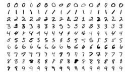
The MNIST digit recognition dataset is a commonly used dataset for benchmarking classification algorithms. The problem consists of classifying a given grayscale image containing a handwritten decimal digit into one of ten classes (from 0 to 9). Each image in the dataset is of size $28 \times 28$ pixels, and the dataset is divided into training and testing sets. The MNIST dataset is particularly useful for testing the performance of different classifiers, such as perceptrons and multi-layer neural networks.

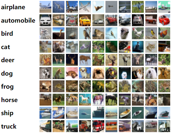
Another example of MEMC classification dataset is the CIFAR10 dataset. The problem consists of classifying a given color image into one of ten classes, such as airplane, automobile, bird, cat, deer, dog, frog, horse, ship, and truck. Each image in the dataset is of size $32 \times 32$ pixels with three color channels (RGB), and the dataset is divided into training and testing sets.