Families of Multiobjective Genetic Algorithms
In real-world optimization problems, it is common to encounter scenarios where multiple conflicting objectives must be optimized simultaneously. This is the essence of multiobjective optimization, where instead of seeking a single best solution, the goal is to approximate a set of trade-off solutions that form what is known as the Pareto front.
To address such problems, several families of algorithms have been proposed, each adopting a different strategy to balance the trade-offs among objectives:
- Pareto-Dominance Based MOEAs: NSGA-II, PAES, SPEA2, etc. These algorithms rely on the concept of Pareto dominance to guide the search.
- Indicator-Based MOEAs: SMS-EMOA, HyPE, CHEA. These use performance indicators, such as hypervolume, to evaluate the quality of solution sets.
- Decomposition-Based MOEAs: MOEA/D, MOGLS, C-MOGA. These break the multiobjective problem into several single-objective subproblems and solve them cooperatively.
Each family brings unique strengths and is better suited to specific problem structures and optimization goals.
🧬 Family I: Pareto-Dominance Based MOEAs
In the field of multi-objective evolutionary algorithms (MOEAs), Family I comprises those algorithms that are based on Pareto dominance. These algorithms aim to construct a set of non-dominated solutions, meaning that no solution in the set is strictly worse than another across all objectives. Well-known examples of algorithms in this category include:
- NSGA-II (Non-dominated Sorting Genetic Algorithm II)
- PAES (Pareto Archived Evolution Strategy)
- Additional variants such as SPEA2, AMGA, AMGA2, and others.
NSGA-II
Motivation and Improvements over NSGA
The original NSGA required additional parameters (e.g., the sigma value for the niching mechanism) and suffered from relatively slow execution. To overcome these limitations, NSGA-II was proposed as an improved version.
NSGA-II features:
- Requires only typical genetic algorithm parameters:
pop_size,n_generations,prob_cross,prob_mut - No additional parameters are needed
- It is elitist, preserving the best solutions found so far
- No external archive is used.
This approach contributes to faster performance and a simpler implementation, as all elite solutions are maintained within the main population rather than requiring a separate memory structure. The elitism mechanism ensures that high-quality solutions are not lost across generations, allowing for a more stable and convergent evolutionary process.
Overview Diagram of NSGA-II Algorithm
The full NSGA-II process is visually represented in the first diagram. It starts with two populations:
P_t: the current generation of parent solutionsQ_t: the offspring generated fromP_t
These two sets are merged intoR_t, which is then subjected to non-dominated sorting. The resulting Pareto fronts (F1,F2,F3, etc.) are used to reconstruct the next generationP_{t+1}by selecting the most promising individuals. The first fronts are added entirely, while the last front (Fv) is partially filled based on crowding distance sorting, ensuring both convergence and diversity. Individuals not selected are discarded (“Rejected”).

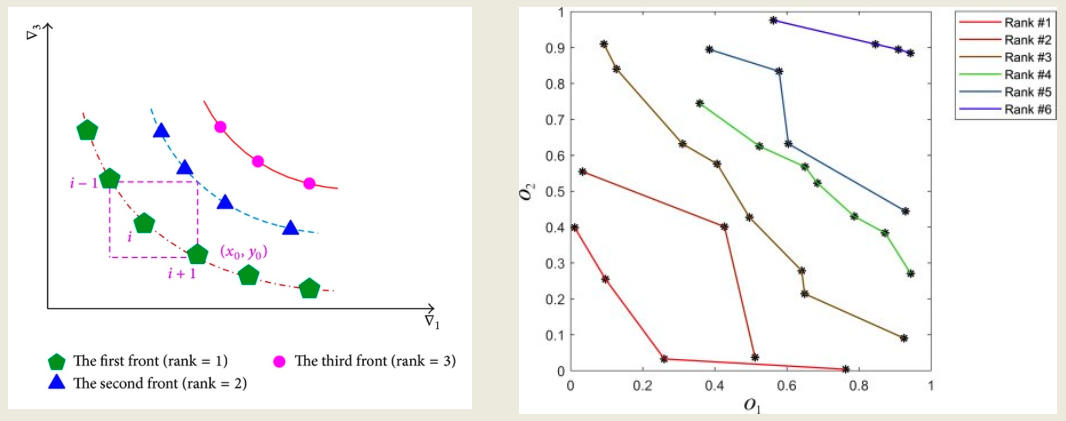
This process of non-dominated sorting assigns each solution a rank:
Rank 1contains all non-dominated solutions.Rank 2includes solutions dominated only by those in Rank 1.- This continues until all solutions are ranked.
On the left of the second image, this is visualized in a three-objective case (v1, v2, v3), while the right side shows 2D ranked Pareto fronts (O1, O2), colored by dominance level. The progression of fronts illustrates how the population is layered in NSGA-II.
Crowding Distance: Formula and Interpretation
Crowding Distance is used to maintain diversity:
- Each front is processed individually.
- Solutions are sorted by each objective.
- Boundary points receive infinite distance.
- Internal points are assigned a crowding score based on the normalized distance between neighbors.
This distance estimates how isolated a point is: higher crowding distance indicates less local competition, making the solution more valuable for diversity.
Crowding Distance MATLAB Code
% Let Fv.f be an L x M matrix with objective values
crowdDist = zeros(l,1);
for m = 1:M
    [sorted_f_m, pos] = sort(Fv.f(:,m));

    crowdDist(pos(1)) = +Inf;
    crowdDist(pos(end)) = +Inf;

    f_m_max = sorted_f_m(end);
    f_m_min = sorted_f_m(1);

    for i=2:l-1
        delta = sorted_f_m(i+1) - sorted_f_m(i-1);
        normalizedDelta = delta / (f_m_max - f_m_min);
        crowdDist(pos(i)) = crowdDist(pos(i)) + normalizedDelta;
    end
end
Data (Fv.f):
Fv.f = [ 3, 11;   % S1
7,  9;   % S2
8,  8;   % S3
11,  5;   % S4
15,  4 ]; % S5
1) Sorting and ranges per objective
Obj1 (ascending): S1(3), S2(7), S3(8), S4(11), S5(15) → range $= 15−3 = 12$ Boundaries: S1, S5 → crowding distance $=\infty$
Obj2 (ascending): S5(4), S4(5), S3(8), S2(9), S1(11) → range $= 11−4 = 7$ Boundaries: S5, S1 → crowding distance $=\infty$
2) Internal contributions per objective $$\frac{f_{i+1}-f_{i-1}}{f_{\max}-f_{\min}}$$
Obj1 (range = 12)
| Solution | Neighbors (Obj1 values) | Raw $\Delta$ | Normalized $\Delta$ |
|---|---|---|---|
| S2 | 8 − 3 | 5 | 5/12 = 0.4167 |
| S3 | 11 − 7 | 4 | 4/12 = 0.3333 |
| S4 | 15 − 8 | 7 | 7/12 = 0.5833 |
Obj2 (range = 7)
| Solution | Neighbors (Obj2 values) | Raw $\Delta$ | Normalized $\Delta$ |
|---|---|---|---|
| S4 | 8 − 4 | 4 | 4/7 = 0.5714 |
| S3 | 9 − 5 | 4 | 4/7 = 0.5714 |
| S2 | 11 − 8 | 3 | 3/7 = 0.4286 |
3) Sum of contributions (total crowding distance)
| Solution | Obj1 | Obj2 | Total |
|---|---|---|---|
| S1 | $\infty$ | $\infty$ | $\infty$ |
| S2 | 0.4167 | 0.4286 | 0.8453 |
| S3 | 0.3333 | 0.5714 | 0.9047 |
| S4 | 0.5833 | 0.5714 | 1.1547 |
| S5 | $\infty$ | $\infty$ | $\infty$ |
Interpretation. Boundary points (S1, S5) get $\infty$ and are kept for diversity; among internal points, S4 is most isolated (highest distance), then S3, then S2.
Note on “more than two” boundary points. Boundaries are assigned per objective. If the min/max in Obj1 don’t coincide with those in Obj2, more than two solutions can receive $\infty$. Tiny sketch:
S1 = (1, 5)   → min in Obj1
S2 = (9, 1)   → min in Obj2
S3 = (9, 9)   → max in both
Here, Obj1 boundaries: S1, S3; Obj2 boundaries: S2, S3 → S1, S2, S3 all get infinite crowding distance.
Main Loop of NSGA-II
P0 = random_generation_of_the_initial_population(pop_size)
Q0 = generate_offsprings(P0) // here we apply the recombination operators

For t=1:max_gen:
    Rt = Pt ∪ Qt
    F = fast_non_dominated_sort(Rt)  // F = (F1, F2, F3, ...)
    Pt+1 = ∅; i = 1                  // the empty set

    While |Pt+1| + |Fi| ≤ pop_size:
        Pt+1 = Pt+1 ∪ Fi
        i = i + 1
    End

    compute_crowding_distance(Fi)  // compute the crowding distance for all the elements in the last front to be added

    k = pop_size - |Pt+1|         // k is an integer value, sayig how many elements are still missing

    Pt+1 = Pt+1 ∪ best_k_elements_in(Fi, k) // the best are the ones having the highest crowding distance

    Qt+1 = generate_offsprings(Pt+1) // here we apply the recombination operators

End
This loop clearly shows how the next generation Pt+1 is built: by including full Pareto fronts until the capacity is almost reached, and then choosing the most diverse solutions from the last partially accepted front.
Fast Non-Dominated Sort: MATLAB Example
This function sorts in fronts the solutions having objective functions in the matrix mat. This functions assumes that all the objectives must be minimized.
Input: mat, an N-by-M matrix, where N is the number of individuals in the current population and M is the number of objective functions (N is the pop_size).
Output: R, a vector of N integers, of the form [ 3 4 1 1 2 3 4 ], saying that the first solution belongs to the third front, the second to the fourth, the third to the first, and so on.
function [R, number_of_fronts] = fast_non_dominated_sort(mat)
    [N, M] = size(mat);
    R = zeros(1, N); % Vector containing the rank of the front for each point
    current_front_index = 1; % Index of the front to consider in the while loop
    F = false(N, 1);
    already_assigned = false(N, 1);

    while sum(already_assigned) < N
        for p = 1:N % p is an index relative to the matrix

            if already_assigned(p)
	            continue;
	        end

            n_p = 0; % Dominator counter of point p (i.e., number of solutions which dominate solution p)

            for q = 1:N
                if q == p || already_assigned(q)
	                continue;
	            end
                if all(mat(q, :) <= mat(p, :)) && any(mat(q, :) < mat(p, :))
                    n_p = n_p + 1; % p is dominated even by q
                end
            end
            if n_p == 0
                R(p) = current_front_index;
                F(p) = true;
            end
        end
        already_assigned(F) = true;
        current_front_index = current_front_index + 1;
    end
    number_of_fronts = current_front_index - 1;
end
This function assigns a front rank to each individual based on Pareto dominance, forming the basis of the sorting phase in NSGA-II.
Final Result
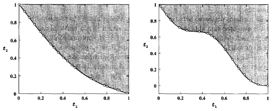
NSGA-II has proven effective at identifying well-distributed Pareto fronts in a single run. As shown in the following image, the algorithm successfully discovers 20 diverse solutions on both convex and non-convex efficient sets, demonstrating its strength in balancing convergence and diversity.
To evaluate the performance of MOEAs, a set of standard benchmark problems is commonly used. These problems typically involve synthetic mathematical functions with known Pareto fronts. They are designed to be challenging by incorporating aspects such as:
- Irregular or discontinuous Pareto fronts
- Convergence difficulties due to deceptive optima
- Complex or high-dimensional input spaces
Most benchmark problems in this context are bi-objective (i.e., with M = 2 objectives), and vary in the number of decision variables (n). These benchmarks provide a controlled environment to test the algorithm’s ability to approximate the true Pareto front in both convex and non-convex scenarios.
| Problem | n | Variable Bounds | Objective Functions | Optimal Solutions | Comments |
|---|---|---|---|---|---|
| SCH | 1 | $[-10^3, 10^3]$ | $f_1(x) = x^2$ $f_2(x) = (x - 2)^2$ | $x \in [0, 2]$ | convex |
| FON | 3 | $[-4, 4]$ | $f_1(x) = 1 - exp(-\sum_{i=1}^3(x_i - \frac{1}{\sqrt{3}})^2)$ $f_2(x) = 1 - exp(-\sum(x_i + \frac{1}{\sqrt{3}})^2)$ | $x_1 = x_2 = x_3$ $\in [-1/\sqrt{3}, 1/\sqrt{3}]$ | nonconvex |
| POL | 2 | $[-\pi, \pi]$ | $f_1(x) = [1 + (A_1 - B_1)^2 + (A_2 - B_2)^2]$ $f_2(x) = (x_1 + 3)^2 + (x_2 + 1)^2$ $A_1 = 0.5 \sin 1 - 2 \cos 1 + \sin 2 - 1.5 cos 2$ $A_2 = 1.5 \sin 1 - \cos 1 + 2 \sin 2 - 0.5 \cos 2$ $B_1 = 0.5 \sin x_1 - 2 \cos x_1 + \sin x_2 - 1.5 \cos x_2$ $B_2 = 1.5 \sin x_1 - \cos x_1 + 2 \sin x_2 - 0.5 \cos x_2$ | (refer [1]) | nonconvex, disconnected |
| KUR | 3 | $[-5, 5]$ | $f_1(x) = \sum_{i=1}^{n-1} -10 exp(-0.2·√(x_i^2 + x_{i+1}^2))$ $f_2(x) = \sum_{i=1}^n (|x_i|^{0.8} + 5 \sin x_i^3)$ | (refer[1]) | nonconvex |
| ZDT1 | 30 | $[0, 1]$ | $f_1(x) = x_1$ $f_2(x) = g(x)·[1 - \sqrt{(x_1/g(x)}]$ $g(x) = 1 + 9·(\sum_{i=2}^n x_i)/(n - 1)$ | $x_1 \in [0,1]$ $x_i = 0$, $i=2,…,n$ | convex |
| ZDT2 | 30 | $[0, 1]$ | $f_1(x) = x_1$ $f_2(x) = g(x)[1 - (x_1/g(x))^2]$ $g(x) = 1 + 9·(\sum_{i=2}^n x_i)/(n - 1)$ | $x_1 \in [0,1]$ $x_i = 0$, $i=2,…,n$ | nonconvex |
| ZDT3 | 30 | $[0, 1]$ | $f_1(x) = x_1$ $f_2(x) = g(x)[1 - \sqrt{(x_1/g(x)}) - \frac{x_1}{g(x)} \sin(10 \pi x_1)]$ $g(x) = 1 + 9·(\sum_{i=2}^n x_i)/(n - 1)$ | $x_1 \in [0,1]$ $x_i = 0$, $i=2,…,n$ | convex, disconnected |
| ZDT4 | 10 | $x_1 \in [0,1]$ $x_i \in [-5,5]$ $i = 2, … n$ | $f_1(x) = x_1$ $f_2(x) = g(x)·[1 - \sqrt{x_1/g(x)}]$ $g(x) = 1 + 10(n - 1) + \sum_{i=2}^n(x_i^2 - 10 \cos (4 \pi x_i))$ | $x_1 \in [0,1]$ $x_i = 0$, $i=2,…,n$ | nonconvex |
| ZDT6 | 10 | $[0, 1]$ | $f_1(x) = 1 - exp(-4x_1) \sin^6(6 \pi x_1)$ $f_2(x) = g(x)·[1 - (f_1(x)/g(x))^2]$ $g(x) = 1 + 9·[(\sum_{i=2}^n x_i)/(n - 1)]^{0.25}$ | $x_1 \in [0,1]$ $x_i = 0$, $i=2,…,n$ | nonconvex, nonuniformly spaced |
PAES
PAES (Pareto Archived Evolution Strategy) is another notable member of the Pareto-dominance based family. It was introduced by Knowles and Corne in 2000 as a second-generation MOEA.
The key differences from NSGA-II include:
- PAES uses an external archive to store non-dominated solutions found during the search.
- It is based on mutation only, rather than crossover and mutation. As such, PAES is categorized as an Evolutionary Strategy (ES).
- In a $(\mu + \lambda)$ Evolutionary Strategy, $\lambda$ offsprings are obtained by mutating $\mu$ parents
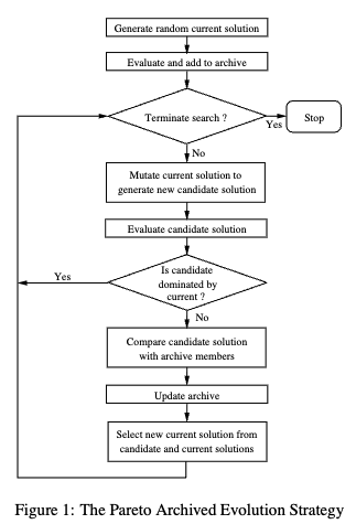
The basic version of PAES is the (1+1) algorithm, where a single parent generates a single offspring through mutation at each iteration. The decision to accept the offspring depends on Pareto dominance and archive diversity:
- Start with a random initial solution $c$.
- Apply mutation to generate a candidate solution $m$.
- Compare the solutions $c$ and $m$ against the current archive:
- If the candidate $m$ is dominated by $c$, reject it.
- Else If $m$ dominates $c$, replace $c$ with $m$, and add $m$ to the archive.
- Else If $m$ is dominated by any archived solution, remove it.
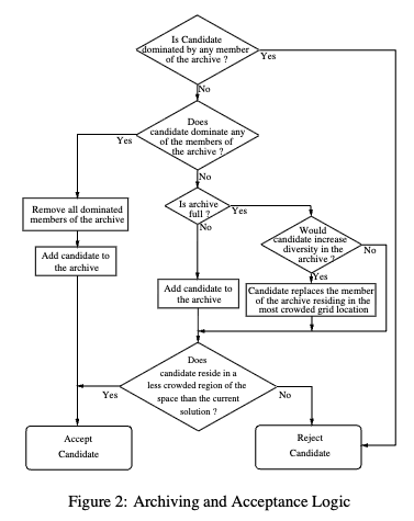
- Else apply the test to $c$, $m$ and the archive to determine which becomes the new current solution and whether to add $m$ to the archive. The test function is the following:
1   if the archive is not full
2       add m to the archive
3       if (m is in a less crowded region of the archive than c)
4           accept m as the new current solution
5       else maintain c as the current solution
6   else
7       if (m is in a less crowded region of the archive than x for
            some member x on the archive)
8           add m to the archive, and remove a member of the archive from
            the most crowded region
9           if (m is in a less crowded region of the archive than c)
10              accept m as the new current solution
11          else maintain c as the current solution
12      else
13          if (m is in a less crowded region of the archive than c)
14              accept m as the new current solution
15          else maintain c as the current solution
One of the main innovations introduced by PAES (Pareto Archived Evolution Strategy) is its crowding handling mechanism based on an adaptive grid built over the objective space. This method offers a compact and efficient way to maintain diversity among solutions without requiring the user to define any niche size in advance.
The core idea is to recursively divide the objective space, which can have multiple dimensions, into smaller and smaller grid cells. When a new solution is generated, its position within the objective space is used to determine its corresponding grid cell. This is done by bisecting the range of each objective recursively: for each objective, the algorithm determines whether the value lies in the left (0) or right (1) half of the interval, building a binary code for each dimension. By concatenating the binary codes for all dimensions, a single binary string is obtained, which can be converted into an integer to identify the solution’s location in a data structure such as a Count[] array that keeps track of the crowding in each cell.
What makes this approach particularly effective is that the grid adapts to the current distribution of solutions in the archive. The grid is recomputed only when the range of objective values changes significantly, which avoids unnecessary updates. This adaptive behavior eliminates the need for a predefined niche size, which is a critical parameter in many traditional niching methods. As a result, PAES achieves both computational efficiency and robustness.
In two-dimensional objective spaces, the adaptive grid can be visualized as a QuadTree, where each quadrant is subdivided recursively to provide finer resolution in regions where more solutions are concentrated. For example, using five levels of subdivision results in 1024 grid cells, since each level multiplies the number of cells by four (1, 4, 16, 64, 256, 1024). Each cell can then be uniquely identified by a binary code of 10 bits, which serves as an index in the crowding array.

To determine the grid location of a solution, one compares its values in each objective to the corresponding ranges, recursively building the binary representation. This binary string is then transformed into a decimal index. For instance, a cell with location 101100 in binary corresponds to a specific index in the Count[1024] array. This allows the algorithm to efficiently keep track of how many solutions occupy each region of the objective space.
This grid-based approach can also be visualized graphically. In two dimensions, it often takes the form of a QuadTree structure, which dynamically refines regions with high density. Such representations highlight how the archive focuses on maintaining resolution where it’s most needed, improving the diversity and quality of the solutions stored.
The (2+2)M-PAES Variant
An important variant of the original PAES is the (2+2)M-PAES, developed in Pisa in 2008. While the classical (1+1)-PAES works by mutating a single solution, this variant introduces the use of crossover to enhance exploration of the search space. In this version, two parent solutions, denoted as c1 and c2, are randomly selected from the archive. These two parents undergo a crossover operation to produce two offspring, which are then mutated, resulting in two new solutions k1 and k2.
The offspring are then compared to the parents to determine which solutions should be preserved. This version is particularly useful in contexts where crossover is beneficial for exploring the solution space more effectively than mutation alone.

The test procedure for the (2+2)M-PES is the following.

Although the adaptive grid provides an elegant and flexible solution for managing diversity, it can become cumbersome to implement and manage, especially in high-dimensional or dynamic objective spaces. However, in situations where the objective space is known in advance, PAES and its variants—such as the (2+2)M-PAES—prove to be especially effective. A typical example is optimization in the ROC (Receiver Operating Characteristic) space, where the structure of the objective space is predefined and stable.
🧬 Family II: Indicator-Based Multi-Objective Evolutionary Algorithms (MOEAs)
Indicator-based MOEAs form a large and widely used family of algorithms in multi-objective optimization. Unlike classical Pareto-based methods, these algorithms rely on performance indicators to guide the selection process. The most common of these indicators is the hypervolume, a metric that quantifies the volume of the objective space dominated by a set of solutions. Among the many algorithms in this family, some of the most representative are SMS-EMOA, HypE, FV-MOEA, and CHEA—each introducing unique innovations based on how they compute or approximate this indicator.
SMS-EMOA
One of the earliest and most influential algorithms in this category is SMS-EMOA, which stands for S-Metric Selection-based Evolutionary Multi-Objective Algorithm. Proposed by Beume, Naujoks, and Emmerich in 2007, this algorithm centers its search process on the direct optimization of the hypervolume indicator—also referred to as the S-metric.
The hypervolume is a powerful metric, but it can be computationally expensive to evaluate, especially as the number of objectives increases. Different definitions and implementations of hypervolume computation exist, offering various trade-offs between exactness and computational cost. SMS-EMOA, however, uses an exact computation strategy.
The algorithm follows a (1+1) steady-state strategy: in each iteration, a single offspring is generated and compared to the current population of size μ. This approach ensures elitism, meaning that the best solutions are always retained in the population. It also inherits the Non-Dominated Sorting strategy from NSGA-II to manage the selection process.
A simplified description of the algorithm’s internal mechanism, including how it selects which solutions to keep when the archive must be reduced, can be found in their paper:
A key characteristic of SMS-EMOA is how it prioritizes candidate solutions during selection. For instance, when choosing among multiple candidates to insert into the archive, those contributing more to the overall hypervolume (i.e., dominating larger regions of the objective space) are preferred. If, for example, solution y8 dominates a larger area than y9, it will be selected over it. This prioritization ensures the population progressively converges toward the Pareto front while maintaining a good diversity.
To better understand the internal functioning of SMS-EMOA, we can now take a closer look at its pseudocode structure. The process is organized around a steady-state evolutionary loop, in which new offspring are generated and integrated into the current population one at a time. Selection is performed using hypervolume contribution as the main criterion.
The general structure of the algorithm is shown in Algorithm 1, which outlines the main loop:
Algorithm 1 – SMS-EMOA
- $P_0 \leftarrow \text{init()}$ /* Initialise random population of $\mu$ individuals */
- $t \leftarrow 0$
- repeat
4. $q_{t+1} \leftarrow \text{generate}(P_t)$ /* Generate offspring by variation */
5. $P_{t+1} \leftarrow \text{Reduce}(P_t \cup {q_{t+1}})$ /* Select $\mu$ best individuals */
6. $t \leftarrow t + 1$ - until termination condition fulfilled
Each time a new offspring is added to the population, the Reduce procedure is invoked to discard one individual and maintain the population size. The core logic of this step is shown in Algorithm 2, which uses fast non-dominated sorting and evaluates the marginal contribution to the hypervolume of each candidate solution:
Algorithm 2 – Reduce(Q)
- ${\mathcal{R}_1, \ldots, \mathcal{R}_v} \leftarrow \text{fast-nondominated-sort}(Q)$ /* All $v$ fronts of $Q$ */
- $r \leftarrow \underset{s \in \mathcal{R}_v}{\arg\min} , \Delta S(s, \mathcal{R}_v)$ /* $s \in \mathcal{R}_v$ with lowest marginal contribution $\Delta S$ */
- return $Q \setminus {r}$ /* Eliminate detected element */
In practical implementations, a slightly simplified version of this logic is often used, especially when dealing with a single non-dominated front. In such cases, if all individuals belong to the same front, the algorithm directly removes the solution with the smallest hypervolume contribution. Otherwise, it removes the one that is most distant from the rest, to preserve diversity. This behavior is captured in Algorithm 3:
Algorithm 3 – Simplified Reduce(Q)
- ${\mathcal{R}_1, \ldots, \mathcal{R}_v} \leftarrow \text{nondominated-sort}(Q)$ /* All $v$ fronts of $Q$ */
- if $v > 1$ then
$r \leftarrow \underset{s \in \mathcal{R}_v}{\arg\max} , d(s, Q)$ /* $s \in \mathcal{R}_v$ with highest distance $d(s, Q)$ */
else
$r \leftarrow \underset{s \in \mathcal{R}_1}{\arg\min} , \Delta S(s, \mathcal{R}_1)$ /* $s \in \mathcal{R}_1$ with lowest marginal contribution $\Delta S$ */
end if - return $Q \setminus {r}$ /* Eliminate detected element */
These algorithmic steps highlight how SMS-EMOA combines exploitation—via hypervolume maximization—with exploration—by maintaining diversity in the solution set.
HypE
HypE (short for Hypervolume Estimation Algorithm) was introduced by Bader and Zitzler in 2011 as a scalable alternative to SMS-EMOA, particularly for many-objective optimization problems where computing the hypervolume exactly becomes prohibitively expensive.
Instead of exact computation, HypE estimates the hypervolume using a Monte Carlo sampling approach. This approximation significantly reduces computational time while still preserving the algorithm’s capacity to drive the search toward regions of high-quality trade-offs.
The key reference for this algorithm is:
The major contribution of HypE lies in making hypervolume-based optimization accessible even when dealing with high-dimensional objective spaces, where traditional SMS-EMOA would become inefficient or inapplicable.
FV-MOEA
FV-MOEA (Fast and Versatile Multi-Objective Evolutionary Algorithm), proposed by Jiang et al. in 2015, represents a further refinement of hypervolume-based optimization. Like SMS-EMOA, it computes the hypervolume exactly, but it improves the efficiency of this process.
The key idea behind FV-MOEA is that, when computing the contribution of a solution to the overall hypervolume, it is unnecessary to compare it against the entire population. Instead, it is sufficient to compare it with nearby solutions in the objective space, thus dramatically reducing the number of computations required.
This insight enables FV-MOEA to retain the precision of exact hypervolume-based selection while being considerably faster than SMS-EMOA.
Reference:
CHEA: Convex Hull-Based Evolutionary Algorithm
CHEA is a distinct member of the indicator-based MOEA family, introduced by a research group in Pisa in 2007. Unlike the others, CHEA does not directly optimize the hypervolume but instead focuses on optimizing performance in Receiver Operating Characteristic (ROC) space—commonly used in binary classification tasks.
More specifically, CHEA seeks to maximize the Area Under the Convex Hull (AUCH) of the ROC curve. This approach is particularly useful when evaluating the performance of classifiers, as the convex hull represents the best achievable performance trade-offs among classifiers in terms of True Positive Rate (TPR) and False Positive Rate (FPR).
This metric is closely related to the traditional AUC (Area Under the Curve) but focuses only on the convex part of the ROC, which corresponds to non-dominated classifiers.
The algorithm and its application are described in:
A typical visualization used in CHEA illustrates how candidate classifiers are positioned in the ROC space. The algorithm identifies and retains those on the convex hull, thus preserving only the most promising trade-offs between sensitivity and specificity. In this context, classifiers not contributing to the convex hull are discarded, as they are outperformed by convex combinations of others.
Here’s the algorithm structure:
- Generate a random initial population $P_0$ composed of $N_{pop}$ solutions and evaluate $FPR$ and $TPR$ for each solution. Create an offspring population $Q_0$ of size $N_{pop}$ from $P_0$ by selecting randomly the mating solutions and then by applying the crossover and the mutation operators. Set $k=0$.
- Evaluate $FPR$ and $TPR$ for each solution in $Q_k$. Build population $R_k = P_k \cup Q_k$. Compute the convex hull, considering always points $(0,0)$ and $(1,1)$, even if no solution in $R_k$ corresponds to these points.
- Assign a rank to each solution. Let $N_1$, $N_2$ and $N_3$ be the numbers of solutions with ranks $1$, $2$ and $3$, respectively.
- Generate the new population $P_{k+1}$ by inserting in sequence:
- Solutions with rank $1$: if $N_1 > N_{pop}$, then randomly extract $N_{pop}$ solutions with rank $1$ and insert them into $P_{k+1}$ and go to step 5; else insert all the $N_1$ solutions into $P_{k+1}$.
- Solutions with rank $2$: if $N_2 > N_{pop} - N_1$, then randomly extract $N_{pop} - N_1$ solutions with rank $2$ and insert them into $P_{k+1}$ and go to step 5; else insert all the $N_2$ solutions into $P_{k+1}$.
- Solutions with rank $3$: randomly extract $N_{pop} - N_1 - N_2$ solutions with rank $3$ and insert them into $P_{k+1}$ and go to step 5.
- If $k = K_{max}$, then STOP; otherwise create an offspring population $Q_{k+1}$ of size $N_{pop}$ from $P_{k+1}$ by selecting through the binary tournament based on ranks the mating individuals and then by applying the crossover and the mutation operators; increment $k$; go to step 2.
🧬 Family III: Decomposition-Based MOEAs
This family of algorithms approaches multi-objective optimization by decomposing the original problem into several simpler sub-problems. Each of these sub-problems is single-objective and focuses on a specific direction in the objective space. The underlying intuition is that, by solving multiple scalar problems in parallel, it is possible to effectively approximate the entire Efficient Frontier of the original multi-objective problem.
Among the most representative algorithms in this family is MOEA/D (Multi-Objective Evolutionary Algorithm based on Decomposition), introduced by Q. Zhang and H. Li in 2007.
MOEA/D: Problem Decomposition and General Idea
MOEA/D transforms a multi-objective problem into N scalar sub-problems, each associated with a different search direction. This direction is defined by a weight vector (also known as a lambda vector), which the user provides. These vectors determine how each sub-problem emphasizes the individual objectives.
Each sub-problem operates in a collaborative setting:
- Every sub-problem maintains its own solution.
- It also shares information with its neighbouring sub-problems, defined by proximity in the weight vector space.
- This allows the solutions of neighboring sub-problems to evolve together, benefiting from shared search experiences.
MOEA/D keeps track of:
- A current population of size N, one solution per sub-problem.
- An external archive of non-dominated solutions, which grows as new high-quality solutions are discovered.
This external archive makes MOEA/D elitist, as it ensures that the best solutions are preserved across generations.
Decomposition Strategies in MOEA/D
Weighted Sum Scalarization
The simplest decomposition method used by MOEA/D is weighted sum scalarization: $$g^{ws}(x,\lambda)=\sum_{i=1}^{m}\lambda_if_i(x)$$ where $\lambda=(\lambda_1,\lambda_2,…,\lambda_m)$ is a vector of weights with $\lambda_i \ge 0$ and $\sum_i \lambda_i = 1$.
Each sub-problem aims to minimize a different scalarized objective. The solutions collectively form an approximation of the Efficient Frontier, assuming the frontier is convex.
- λ=(1,0): focuses only on minimizing f1
- λ=(0.9,0.1): gives more importance to f1 but still considers f2
- λ=(0,1): focuses only on f2
Chebyshev Scalarization
To overcome the limitations of the weighted sum (especially in non-convex frontiers), MOEA/D can also use Chebyshev scalarization: $$\min g^C(x|\lambda, z^)$$ $$g^C(x|\lambda, z^) = \max{\lambda_i \cdot |f_i(x) - z^*_i|}$$ where $z^∗$ is the ideal point, i.e., the best (minimal) value observed for each objective across the search, meaning that $z_i < \min f_i$.
This scalarization ensures that any Pareto optimal solution can be found by an appropriate choice of λ. However, it has a non-smooth formulation, which may be problematic for gradient-based optimization methods.
Neighbourhood Structure
In MOEA/D, neighbourhoods are defined in the space of weight vectors. Two sub-problems are considered neighbors if their weight vectors are close in Euclidean distance.
This is based on the assumption that nearby sub-problems correspond to similar trade-offs and likely share similar optimal solutions. This proximity enables:
- Local information sharing
- More coherent evolutionary pressure
- Efficient diversity preservation
Collaborative Solving: Evolution and Replacement
At each generation, MOEA/D performs the following steps for every sub-problem:
- Mating Selection: Solutions are selected from the current neighborhood (including the current solution of the sub-problem) to generate offspring.
- Reproduction: Genetic operators (e.g., crossover and mutation) are applied to create a new candidate solution.
- Replacement:
- The new solution replaces the current one if it improves the sub-problem’s scalar objective.
- Additionally, it may also replace some of the neighbors’ solutions if it performs better under their respective scalarizations.
This leads to an implicit cooperation between sub-problems.
MOEA/D: Pseudocode (High-Level Description)
Input
- Multi Objective Problem
- N: number of sub-problems
- ${\lambda_1, \lambda_2, …, \lambda_N}$: set of N uniformly distributed weight vectors
- $T$: The neighborhood size (NS)
Initialization
- Compute the Euclidian distances between any two weight vectors and then determine the $T$ closest weight vector to each $\lambda_i$. For each $i = 1, …, N$, set $B(i) = {i_1, …, i_T}$, where $\lambda_j, \forall j \in B(i)$ are $T$ closest vectors to $\lambda_i$
- Generate initial population randomly
- Evaluate $F(x_i)$ $\forall i = 1, …, N$
- Set ideal point $z^* = \min(f_1(x), …, f_m(x))$ over all $x$ in the population
Evolution (repeated until stopping criterion)
For each sub-problem $i = 1, …, N$:
- Randomly select two indices $k$ and $l$ from $B(i)$, and generate a child solution $x_{child}$ from parents $x_k$ and $x_l$ by applying genetic operators.
- Repair $x_{child}$ by applying problem-specific repair/improvement heuristic.
- Evaluate $F(x_{child})$
- For each $j=1, …, m$, if $z_j > f_j(child)$ then set $z_j = f_j(child)$.
- For each neighbor $p$ in $B(i)$, set $x_p = x_{child}$ and $F(x_p) = F(x_{child})$ if $g^C(x_{child}| \lambda_p, z^) \le g^C(x_{p}| \lambda_p, z^)$
Termination
- Output the final population as the Pareto Set approximation
- Use $F(x_1), …, F(x_n)$ to approximate the Efficient Frontier
- It naturally divides the problem into simpler components.
- It promotes both diversity (via neighborhood structure) and convergence (through elitism and scalarization).
- It can be extended with different decomposition methods, selection mechanisms, and local search strategies.
📊 Comparing the Performance of Two MOEAs
When evaluating and comparing the performance of two Multi-Objective Evolutionary Algorithms (MOEAs), it is essential to rely on quantitative performance indicators. These metrics aim to assess the quality of the approximation that a given MOEA produces of the Pareto front.
Several commonly adopted indicators include:
- Hypervolume
- Generational Distance (GD) and its variant GD+
- Inverted Generational Distance (IGD) and its variant IGD+
- Delta Metric: defined as the maximum between GD and IGD (or GD+ and IGD+ in the improved version)
Generational Distance (GD)
The Generational Distance (GD) metric evaluates how far the solutions found by a MOEA are from the true Pareto front. Let:
- $A={a_1,…,a_n}$ be the set of non-dominated solutions produced by a MOEA.
- $Z={z_1,…,z_m}$ be a reference set representing the true Pareto front.
- $d_i$ be the Euclidean distance between a solution $a_i \in A$ and the closest solution in $Z$.
- $p$ be a norm parameter, usually set to 2 (i.e., Euclidean norm).
The GD metric is defined as: $$GD(A)=\frac{1}{n}\left(\sum_{i=1}^n d_i^p\right)^{1/p}$$ A lower GD indicates that the solutions found by the algorithm are closer to the true Pareto front.
Inverted Generational Distance (IGD)
The Inverted Generational Distance (IGD) performs the inverse of what GD does: it measures how well the true Pareto front is represented in the set of solutions found by the MOEA.
Formally:
- Let $d_i$ now represent the distance from a reference point $z_i \in Z$ to the closest point $a_j \in A$.
- Then: $$IGD(A)=\frac{1}{m}\left(\sum_{i=1}^m d_i^p\right)^{1/p}$$ This metric indicates coverage: how well the algorithm’s solutions represent the true front.
Delta Metric ($\Delta$)
To provide a single performance value that accounts for both proximity and coverage, the Delta metric is defined as: $$\Delta(A)=\max{GD(A),IGD(A)}$$ Lower values of $\Delta$ correspond to better performance.
Hypervolume (HV)
The Hypervolume indicator, as already discussed in algorithms like SMS-EMOA, computes the volume of the objective space dominated by the set of solutions A, bounded by a predefined reference point.
- It captures both convergence (how close solutions are to the Pareto front) and diversity (how well they spread across the front).
- It is the only unary indicator that is strictly Pareto compliant.
Computing the hypervolume can be done:
- Exactly, using geometric algorithms (feasible in 2D and 3D)
- Approximately, using Monte Carlo sampling
Summary
| Metric | Purpose | High Value Means | Low Value Means |
|---|---|---|---|
| GD | Proximity to front | Far from front | Close to front |
| IGD | Coverage of true front | Poor coverage | Good coverage |
| $\Delta$ | Worst of GD and IGD | Weak overall quality | Good balance |
| HV | Volume dominated | Good coverage + conv. | Poor overall quality |
These metrics are complementary, and no single one gives a complete picture. A proper evaluation of MOEAs should consider multiple indicators for a more robust and fair comparison.